Breaking Exogenous Characteristics

How can we study the creation of new products?

In industrial organization, one of the most standard assumptions is that the characteristics of a product are exogenous. This means we take them as given, and we do not inquire into why they are how they are. There are two basic reasons for this. First, having product characteristics be exogenous is enormously helpful when it comes to actually estimating demand. For technical reasons, which I will explain later, assuming product exogeneity is sufficient variation to identify your model. Without it, you would need two sources of instrumental variables.

Second, and perhaps more importantly, endogenizing product characteristics is really hard. It is not always clear that the question of where firms place their products can ever be satisfactorily answered for many industries; assuming that they have been placed, and all we need to worry about is pricing, is greatly simplifying, and in many cases a good enough approximation. However, it is just that – an approximation – and it can matter empirically, as we shall see by way of an extended example.

Consider the ready-to-eat cereal market, which are things like Frosted Flakes, Cheerios, and Apple Jacks. Economists have written a lot of studies on this industry (notably, Schmalensee (1978), Hausman (1996), Nevo (2001), and Backus, Conlon, and Sinkinson (2021)) because it has a lot of nice properties to demonstrate techniques on. (There are many varieties, but only a few firms, all of whom are publicly traded, and we have excellent data, including detailed data on what products consumers actually buy).

Backus, Conlon, and Sinkinson (2021) use this industry as a way to test in miniature a story that, if true, would have enormous implications. In the past few decades, large institutional investors like Vanguard, Blackrock, and State Street have come to control a small but substantial part of many different companies. This leads companies to no longer necessarily want to maximize their own profits – instead, they may care about the profits of other companies a bit as well. Given some set of products, this would lead them to charge higher markups and compete less aggressively than they otherwise would.

There are three things we don’t know: conduct, costs, and demand. We don’t know the manner in which firms compete with each other – whether they are colluding or maximizing their own profits or somewhere in between – and that is the question we are trying to answer. We don’t know the marginal cost of producing a unit of cereal. We do not know how consumers value different goods as a function of their characteristics.

The demand system is the first thing we seek. We’re gonna build this one up, starting from a logit model, and then on to random coefficients. If we only cared about exactly one good, then we could easily get this with an instrumental variable – something which shifts supply without shifting demand. Imagine, for instance, that the sugar is affected by the weather, but the weather does not affect the demand for sugar. Then we can simply trace out observed prices and quantities after using the weather as a first stage, and that’s our demand curve. However, when we have many goods, the price and quantity purchased depends on the price and quantity of every other good in the market. Instead of J instruments for J goods, we need J squared instruments.

Suppose that consumers buy one good out of many options, and get utility from the characteristics of the good X, disutility from the price, p, and utility from an unobserved quality component ξ, plus an idiosyncratic error term with a Type I Extreme Value distribution. The error term makes it so we have a very convenient solution when we plug in the market shares of each good, and we can compute it in milliseconds.

Unobserved quality, which we can think of as a brand name, the taste of a product, or simply any characteristic which is not in our vector of characteristics X, is unobserved by us but is observed by the market participants, will be correlated with price. Thus, we still need an instrument. Neatly enough, though, the exogenous characteristics is an instrument, since we assumed they are uncorrelated with unobserved characteristics.

The drawback to logit is that we have very restricted substitution patterns – there is no concept of goods being more or less similar. So what we do instead, ever since Berry-Levinsohn-Pakes (1995), is allow there to be a distribution of consumer preferences for each characteristic. Each person draws from that distribution. The mean of each distribution governs total demand for products in that industry, versus those outside the industry, and the variance tells us how much consumers disagree in their valuations, and thus how they will substitute to other products.

As with logit, we will need an instrument in order to shift the price without shifting demand. However, in addition, we will also need another instrumental variable to pin down the variances. Exogenous product characteristics are very convenient for this, because if there is variation in product availability across markets, then we can use the similarity of products to see how people substitute from one to another.

Unlike logit, there is no closed-form solution, where we can just plug in market shares and go. Instead, we need to find the optimum via iteration. We start by taking a guess at the parameters which govern the variance for each dimension of product quality, and then we solve for the means of the distributions which justify the market shares we observe. Then we go back, and see how much it correlates with our instrumented prices. We take another guess at the variances, and repeat this exercise until we arrive at something close to optimum.

What makes this possible is that the inner loop, the solving for the means, will eventually converge to a single optimum. If you run it over and over, you will converge upon a definite answer. So you do it out to 12 decimal points, and that’s good enough for the outer loop, which is guessing the variance. This nested fixed-point loop originates from Rust (1987), and if you want to actually run it yourself, the industry standard is PyBLP by Conlon and Gortmaker (2020).

So far we’ve assumed that the distributions are parametric, which is to say that they follow distribution, but we can identify the model more flexibly if we have microdata. BCS have data from Nielsen on who purchases which cereals, which allows them to see how preferences vary with things like the number of children in a family. You can allow for distributions like bimodal, which might be the case if some people with kids really like Lucky Charms, and people without kids really dislike Lucky Charms. (The first person to do this was Amil Petrin (2002), who studied the introduction of the minivan – yet another good where consumer demand will depend starkly on the number of kids!).

Now we have a complete demand system. Ordinarily, we get marginal costs by first solving for a demand system, assuming a mode of competition, and then showing what marginal costs would have to be to justify the prices we observe. We can’t do that, of course, because conduct is the question. The last time someone tried to test conduct in the breakfast cereal market (Nevo, 2001), he took estimated markups from accounting data, which unfortunately have very little to say about what the markup actually is. (If only it were so easy to observe marginal costs!). Conduct is not identified separately from marginal cost, because there is always a combination of costs and conducts which can justify the observed prices.

The first person to take a crack at solving for conduct was Bresnahan (1982), who suggested using instruments which would “rotate” demand, such as changes in the price of close goods; BCS use an innovation from Berry and Haile (2014) which is more general. Let’s say that consumer demographics are exogenous. If we are observing the true model of conduct, then if we subtract out the true markup the marginal cost left over should not be correlated with demographics. If it is, then we have the wrong mode of conduct! How they check for correlation is a bit beyond this blog post, but it’s random forest – any flexible, nonparametric estimator will do. They do not rely on just demographics, of course – they use several sets of excluded instruments, and argue that since they all have different assumptions needed for it to work, but they all agree, the underlying model is correct.

After doing all this, they find that the model which best fits the data is that firms are maximizing their own profits, rather than maximizing their joint profits under common ownership or maximizing their joint monopoly profits. We can breathe a sigh of relief, though we should not rest easy; were they to exercise their latent market power and maximize their profits according to common ownership, prices would rise around 5%. For the purpose of comparison, if the firms were to act as a collusive monopoly, prices would rise by 10%.

The trouble with this is that taking the placement of products as exogenous rules out one of the biggest margins along which firms might collude. Firms could place their products in such a way as to advantage their other holdings. Much of the earliest literature on the breakfast cereal market alleged that the main companies were deliberately creating too many products to prevent the entry of competitors, and then charging higher markups.

In 1972, the FTC brought suit against the major manufacturing concerns (excepting Quaker Oats, who was dismissed from the case) about exactly this. A blow-by-blow view of the case is given by F. M. Scherer (2013), who worked for the FTC at the time; Richard Schmalensee (1978) can be taken as an official statement of the FTC’s economic reasoning behind the case. We should introduce a way of thinking about product positioning now, which I have been occasionally hinting at whenever I say “where” in reference to products. Think of a line in space, like a beach. There are some number of ice cream shops. Each person on the beach faces some cost which is quadratically increasing in distance from where they are to the ice cream stand. Each ice cream stand can then, if people are uniformly distributed, increase their profits by spreading out from other firms.

Back to Schmalensee. Each new product line requires a fixed cost to enter. Because the firms are producing many varieties, any new entrant is only willing to enter if they have sufficient space on the line to enter. If the firms are colluding, they will create too many products to crowd out competitive entrants, and then charge higher markups. The point of product differentiation, instead of threats of price wars, is that the threats are not credible conditional upon someone entering. Once they enter, the incumbents would prefer to work with them rather than against them. By contrast, the product line is going to stay there and will continue to reduce competitor profits.

We could tell a story in which the companies can’t collude on price, but they can strategically coordinate where they place their varieties. Perhaps sticking to a collusive agreement would be too hard and inevitably attract the attention of the competition authorities, but the placement of products would be a fait accompli and credibly commits them to a particular area. Then firms could position themselves such that no one would have quite enough room to enter, but they would be able to collect higher markups and profits than if they were competing fairly.

I should note that this is not quite the same story as Schmalensee (1978), who is considering a model where they do indeed collude. It is not at all clear whether firms, if they were colluding, should place their products closer or farther apart. The case for placing them farther apart is easy to see – if consumers have fewer close substitutes in terms of characteristics, the firms will be able to charge a higher markup for those goods. The case for packing them in together, though, is to keep other possible competitors from entering. Without knowing the characteristics of potential entrants, we can hardly compare the optimal behavior of even a monopolist producing many varieties to the observed varieties. There is work on radio stations by Berry and Waldfogel (2001) of particular relevance, who show how mergers among radio stations led to more stations, so as to preempt competitor entry.

I do not think that anyone has come to a perfectly satisfying answer as to how to endogenize product characteristics. However, some people have tried. The remainder of this essay will review what people have done, at considerable length. I will then discuss how convinced I am by this, and what we can take away. Before the papers, two general notes:

As a general rule, the first step is to rule out actually shifting the characteristics of a product. Instead, you have to introduce a product line, which cannot be shifted afterwards. Otherwise, it’s simply not plausible we would reach an equilibrium. We can analogize to voting, where we think of candidates as having positions in issue-space instead of product space. The McKelvey-Schofield chaos theorem shows that in most cases, no equilibrium outcome exists if people are able to costlessly and sequentially change their positioning. If we are going to allow for the product characteristics to be changed, rather than having an entry game, it must be once and for all.

We then generally need some sort of trick to simplify the computation. Including everything, and making everyone’s actions depend upon everyone else’s actions, blows up the number of things we need to compute. Much of the discussion in the upcoming papers will be on what, exactly, the computational trick is.

We’re first going to cover a study where entry is taken for given, and quality is a continuous choice. Ying Fan (2013) is studying the newspaper market, and evaluating what might have happened had several prospective mergers gone through. Because of this, she can use demographic characteristics as instruments, in two ways. First, since we have taken the geographic placement of the newspaper as given, the observed preferences of different demographics directly shifts what the newspaper will offer. Then, the demographics of the places served by newspapers which are partially overlapping in coverage affect the quality the newspaper will offer, but only through its effect on the competitor’s characteristics. She limits the number of firms in competition to a few major markets, so as to prevent everything from depending on everything, and

In stage 1, everyone chooses the characteristics. Then in stage 2, everyone chooses the price of a subscription and the advertising rate. You could estimate it by iteration, where you take a guess at characteristics, then solve for prices, and work backwards until you get a maximum, but this would take too long. The main estimation trick of the paper is that she takes the second derivatives of the pricing equations, and uses that to tell her where what the marginal benefit of a change in quality would be. If the curvature of the functions in the model is correct, then she can use that without needing to establish what the effect of changing the quality would be by iterating.

When she applies this to some counterfactuals, she finds that endogenous quality adjustment will lead us to understate the welfare harms of the tested mergers. It is unfortunate that the mergers were not consummated, as it would be nice to compare to the ground truth. The particular instruments she uses – what are sometimes called Waldfogel instruments – are limited to spatially segregated markets. There is no variation if firms serve a national consumer base.

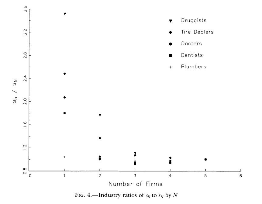
There are a number of other studies which use geographic segmentation to infer things of importance. Most of these are dealing with entry, however, and so make different simplifying assumptions, and commonly compress the heterogeneity of firms or products. Bresnahan and Reiss (1991), which is a certified classic by the way, studies the entry of additional businesses, like doctors and dentists, into these extremely isolated Western towns. We can see that as the town increases in size, more firms will enter, but that the number of additional people needed for each new firm is also increasing – the only plausible presumption being that additional entrants toughen up competition and reduce the profit margins available. However, we have to explicitly assume that firms are identical.

Berry (1992), who is studying entry into particular airport to airport hubs, also assumes a lot of homogeneity – firms can have different fixed benefits to already having lots of flights going to and from an airport – but no difference in the variable profits is allowed. In Mazzeo (2002), otherwise identical firms simultaneously choose where to enter the level of quality of their product, discretized into three bins. The computational “trick” in Mazzeo is simply that the number of possible product types is incredibly limited.

I prefer Seim (2006), who estimates the geographic placement of video stores, but the methodology is general. If all firms possess all information, then computing an equilibrium requires showing that there is no unilateral deviation which is profitable. This is, of course, computationally costly. Her response is to give the firms private information about their productivities, which actually makes choosing a strategy for competing firms easier. There’s just a distribution, and you randomize. Her method is only used for geographic placement, but can be used for anything we think of spatially, including product characteristics as mentioned before. Draganska, Mazzeo, and Seim (2009) also is estimating an incomplete information game, for the same reasons.

Eizenberg (2014) studies the development of computers in the PC market under complete information, with the methodological contribution being partial identification. You say that the profits of offering a product are decreasing in the number of competitors. Thus, observing it with many competitors, and not observing it with few, give you bounds on the fixed costs which can justify it. This allows him to prune products which a firm would never offer, even in the best of circumstances.

Thomas Wollmann (2018) has a paper studying the entry of new product varieties in the commercial vehicles market. In this industry there has been no change in the major firms in decades. What change there is has come through changes in the product lines available.

Here the computational trick is kind of a hack. He just asked experts in the industry what the approximate cost of introducing a new variety would be, and used that for an estimate of costs. It’s called a “hurdle rate”. Basically he argues that the computational burden for optimally introducing new products is so extraordinarily large that not even the firms themselves can do it. I see echoes of Benjamin Moll’s criticism of rational expectations in heterogeneous agent macro – if we can’t solve a Bellman equation with billions of dimensions, neither can the agents. (To be clear, this is conceptually different from much of the computational difficulties which motivate our modeling choices! In most cases, the right decisions are easy to know if we know our own costs, and it’s inferring those costs which is computationally difficult. Here, though, the right decisions are not clear without complicated optimization). Instead, planners follow a rule of thumb, where they enter if and only if there is an expected minimum rate of return, considering only their own position and not the response of others. This means that each firm only has to solve one thing, and you can cleanly and simply identify things.

The practical upshot of assuming the hurdle rate for decision making is that you can allow firms to perfectly observe others’ cost shock. You don’t need everything else.

Alejandro Sabal (2024) studies product entry in the passenger vehicle and light truck industry, and so is a sort of companion to Wollmann’s paper. (In prior work, the famous Berry-Levinsohn-Pakes (1995) paper was on the automobile industry, and Grieco, Murry, and Yurukoglu (2024) is worth reading as a sterling example of doing absolutely everything you can do in BLP type demand estimation, without endogenizing the product characteristics).

Sabal’s paper has a lot of contributions, though, and I do not want to belittle it by making it no more than a companion. In fact, I think it ties everything together. Firms engage in a three stage game, working backwards to solve the model. In stage three, companies are aware of demand, which is estimated with the standard mixed-logit methods discussed at length earlier in the post. Firms can also work out which markets they would enter, given the demand they observe. In the first stage, each firm gets a set of shocks to the fixed cost of removing or creating any new products.

Rather than work out the exact solutions to anything, because with 20 choices and 10 firms he would need to check 10^60 different entry configurations, he instead gets bounds from a property which seems sensible (but is not yet satisfactorily proven): the marginal value of adding one additional product is decreasing in the number of products offered. He can get an expected value for a firm with one product, and a firm with many products, and show that the fixed costs must be between the two extremes. This is the partial identification used by Eizenberg.

I find myself very excited by the possibility of endogenizing product characteristics via estimating a game. Excited, however, does not mean convinced. The features of your model that are driving the result often remain opaque; you often have no idea whether the model is correctly specified or not. There is no way either to avoid unrealistic assumptions. Maybe you think exogenous product characteristics is a bit unrealistic – but is it really that much more unrealistic than what you would have to believe to compute the dynamic model?

Even if your model is correct, these papers take an enormous amount of time to do. Conversations with staff at the FTC indicate that they are already unable to apply the most advanced methods as much as they want to due to the time constraint; at times these papers are mergers which were considered but never done long ago (Fan, 2013) or on whole industries that went extinct not long after (Seim, 2006). For considerations of product entry to be meaningful, we have to turn it into a consistent sign or bias. Most of what Hendel and Nevo (2006) taught us, practically speaking, was not that we would need to compute a dynamic game every time a good is storable, but simply that we should expect the demand elasticities to be biased in one direction, and so we should both take the estimates with a grain of salt and insist upon aggregation over longer time periods.

I do think it suggests a skew toward thinking mergers are more dangerous to the consumer than before, because price is not the only margin on which they can disadvantage the consumer; this is especially the case if you expect price to be easier to measure than product quality. Other than that, I have no universally applicable conclusions.

One thing, however, is clear. If you want to do this – go to Yale! Berry and Haile lurk.