Everything I Know About Dynamic Discrete Choice

Rust 1987

I do not think anyone understands quite what John Rust is doing the first time they read Rust (1987). I certainly didn’t. It was only upon seeing it applied elsewhere, and being given a high level overview, that I could approach the forbidding cliffs and begin to scale them. In this essay, I am going to give you crampons and an ice ax, then discuss the wonderful map of everywhere you can go with dynamic discrete choice models.

Mr. Harold Zurcher is the superintendent of maintenance for the Madison Metropolitan Bus Company. The Bus Company possesses 162 buses, largely purchased from the General Motors Corporation, all of which are diesel powered and run for about 5000 miles every month. Mr. Zurcher’s goal is to maintain the buses in such a way as to maximize the profits of the Bus Company, bearing in mind not only the cost of repairing or replacing the engines, but also minimizing the loss of consumer goodwill which a breakdown would cause. The data we have are monthly readings of the odometer, and a record of the date, mileage, and maintenance actions when the bus went into the shop. Our task is to infer the underlying cost functions using only his decision to replace and not replace.

You might ask why we do not simply phone the General Motors Corporation and ask them ourselves what the cost of replacing a bus engine would be. We will need to do something like this, in order to convert our measurements of ratios into dollars, but just doing this would be missing the point. Here, we might have an answer key, although of course the engine itself is only part of the cost of taking the bus out of service, and Mr. Zurcher generally rebuilds a new engine completely out of parts. In many other contexts, we will not have this. We need to find the underlying cost functions using the data which we have, not the data we wish we had.

I will give the high-level overview of solving the problem first, and then expand upon each of the details. Every month, Mr. Zurcher decides whether to replace the bus engine, or to continue to the next period without replacement.. We can see immediately that any model with a deterministic stopping point at which the engine is replaced would be rejected. The exact mileage at replacement varies considerably. Note that we are chunking the mileage into 90 bins, one for every 5,000 miles.

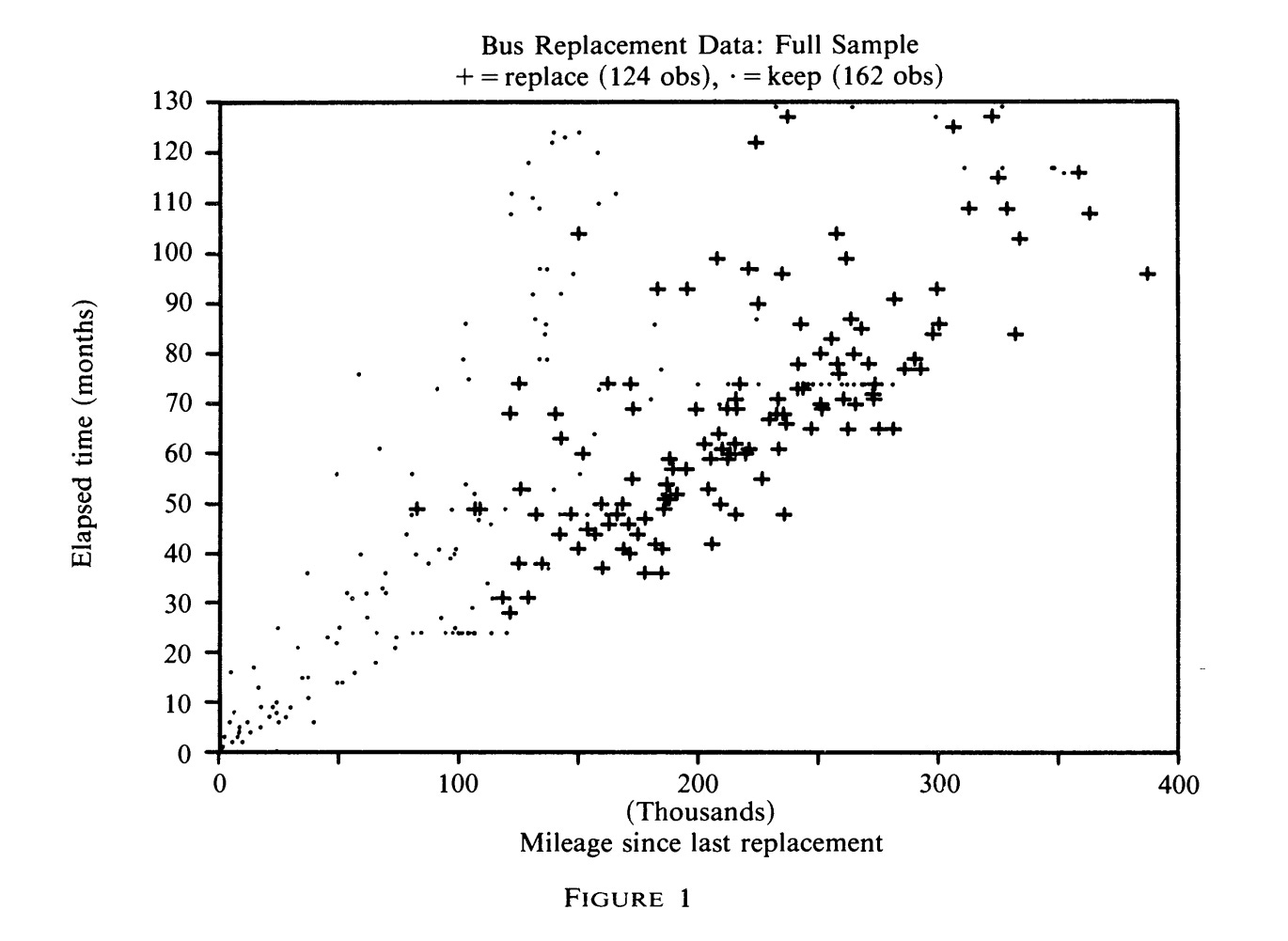
What we will instead do is allow for there to be idiosyncratic shocks to Mr. Zurcher’s decision to replace the bus. He is an expert in the ways of buses, so it stands to reason that sometimes he will see that an engine is holding up well, and other times it isn’t. These are errors are not correlated with each other over time, but drawn anew each time the bus comes into the shop.

These shocks have a very particular structure – Type I extreme value errors, called logit. Why this? Why not a normal distribution? Put plainly, it makes computation more simple later on. More specifically, because the logit distribution is built around e, the probability that an engine is replaced is equal to e to the power of the value of replacing, divided by the sum of all e to the power of every other option. This gives you a number between 0 and 1, which you can read off as a probability. A normal distribution for idiosyncratic shocks would require some extraordinarily nasty integrals.

So once again, we take a guess at the outside parameters. We impose a discount factor, so that Mr. Zurcher values the future a little bit less than the present, and try a replacement cost RC, and a function of ongoing costs as a function of mileage. This will converge to a fixed point, a set of 90 values, one for each bin, with a percentage likelihood of replacement which maximizes Mr. Zurcher’s expected utility. We can then compare the optimal replacement, given these costs, to the actual replacement. If they aren’t close enough, we try a new set of costs, and do this iteration over and over again until we have an answer.

I think we should be clear about what this fixed point is that we’re iterating to. A fixed point is simply some value which, when plugged into an equation, returns itself. For instance, the function f(x) = x^2 has fixed points at 0 and 1. We’re looking for a set of 90 numbers, one for each bin and denoting the present discounted value of being in that state, which when fed into the Bellman operator gives us the same vector of 90 numbers.

What is this Bellman operator? We hand it the vector, and it considers the possibility you land in each future state. (We get this from the data – this just means what the mileage will be a month from now). For each of these, we have our current guess of the expected value of being in that state. We use the logit error formula to get the value of being in each state, given optimal play, then weight going from state to state by the likelihood of doing so in the data.

These guesses will almost certainly be wrong! They are wrong because they are inconsistent with each other. If costs are increasing as a function of mileage, for instance, the value of being in lower mileage states should be higher. But we can use them to find the right guesses.

We take our current guess. We plug it into the Bellman operator. It spits out what the “real” value of being in that state would be, given what our other guesses is. We subtract the “real” values from the first guess, and are left over with a residual. This residual tells you how off you are at each guess.

Each state has a connection to every other state, so there are 90 by 90 values denoting exactly how much each state affects every other state. If you take the inverse of this matrix, the Jacobian, you can multiply it by the vector of leftover values – the residual – and after subtracting this new, updated matrix from the current guess, you get a new guess. The Jacobian is translating that residual into a coordinate update of all of the cells at once. You compute a new Jacobian each time, and the stuff you did in calculating the likelihood of going from state to state provides weighting for each cell in the Jacobian. Every time you do this operation, you double the number of correct digits, and converge very close to the correct answer with only a few iterations.

The results do not currently live in the form of dollars, but as ratios of each other. We can convert them into dollars by speaking to Mr. Zurcher, and asking him what he thinks the cost of replacing the bus engine is, which gives us the RC.

There are some things we cannot do with this. We need for there to be some discounting of the future, in order for the expected future value of being in every state to not be infinite. We also cannot identify the discount factor separately from the replacement cost, as any change in the discount factor can be offset by a corresponding change in the replacement cost.

Above all, we are limited in the number of variables we can have, largely because of needing to invert the matrix. Suppose that we wanted to keep track of the age of the bus. For the sake of argument, if we binned it into 90 chunks, then we’d have 90 squared, or 8,100, states. This would mean inverting a 8,100 by 8,100 matrix, which is 90^6 computations. Nowadays you could actually do that, although everything would take annoyingly long, but Claude assures me that on the IBM-PC Rust programmed this on would take 8 days to do one single matrix inversion – little surprise, since it would take about 700,000 times more computation.

You might be wondering to yourself – why? Why do we need all this complex math and incredibly fiddly computation, when we could just solve this with a regression? Take the likelihood of the engine being replaced as a function of mileage, draw a line through it, and call it a day. This might be useful for some applications, but you will find yourself completely unable to answer counterfactuals. What happens if the cost of replacing a bus engine increases, or falls?

Your regression has nothing to say about it. You’ve never seen the bus engine cost vary, so your regression slope is totally uninformative. If you want to accurately assess situations which are not exactly like the variation you see in your data, you need the underlying costs which drive behavior.

Let’s take a look at Vincent Rollet’s job market paper, “Zoning and the Dynamics of Urban Development”. Zoning restricts what types of buildings can be built on different plots of land, in particular the size. Many people have proposed that if we upzoned neighborhoods, rents would fall and welfare would rise. We could measure the effect of upzoning by looking at prices and quantities

But this is such a narrow problem to solve. If we want to evaluate the effects of a rezoning, we would be unable to unless another rezoning of similar characteristics had happened earlier in the data. What’s worse, these small scale regressions cannot actually identify welfare – they can measure change in price, and they can measure change in population, but they cannot really account for building housing in New York will affect the demand for housing across the country.

So instead, Rollet solves for the complete supply and demand system. The demand side is given by a quantitative spatial model, in the vein of Ahfeldt, Redding, Sturm, and Wolf (2015); it, too, won a Frisch medal, and so I will skip over the details in the interest of time.

To get the supply side, Rollet solves an extension of Rust’s model, with an additional loop, to get the building choices of developers. They face a cost to build, which includes the cost of tearing down the building which previously resided on the plot, and can choose to exercise the option to build once. Given the costs we guess in the outer loop, we solve the inner loop for whether the plot will be redeveloped. There is then a middle loop, in which they account for how their decisions will affect the supply of housing in the city and its subsequent price (and they’re forced to be consistent with each other), and we can take another shot at the costs.

If the cost functions are correct, then the effects should track what we observe from quasi-experimental estimates. And indeed they do!

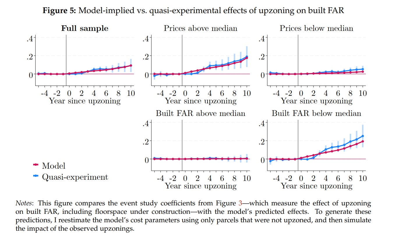
Rollet’s model can tell us things that the quasi-experiments can’t. For example, the amount of housing built after a rezoning will tail off as the rezoned area gets more developed. We would not otherwise be incorporating the cost of tearing down a building, and how that both discourages building where development has already happens, and encourages holding onto underdeveloped land for longer. He also predicts that upzoning New York would mainly affect the population of the city, and not so much the rent. It is the places outside NYC which would see a fall in rents, as people move to the Big Apple.

Similarly, we can look at Aradhya Sood’s “Land Market Frictions in Developing Countries”, who is curious how much the small size of plots in India disrupts manufacturing firms. Records of the price of land in India do not exist at scale. Even if they did, the real cost of land includes negotiating and the landowners holding out for better deals. You have to back out the underlying cost functions if you want to have any hope of answering what would happen if the government made it easier for landowners to pool their land together to sell, or for the government to repeal the 2015 eminent domain reforms.

I have cited these excellent recent papers because they address what I believe to be the strongest criticism of the literature of dynamic discrete choice, whether estimated with methods due to Rust specifically or not.. The papers are, very often, simply not answering a question of interest. Either the process of estimation has taken too long and the questions they study have been long since outmoded, or they have chosen a question with easy data but for which there was never any practical interest whatsoever. The prime example of the former must surely be Stephen Ryan (2012). I note that it is an excellent paper doing interesting things, of course, but it is a paper published in 2012 evaluating the effect of a policy change in 1990, long after it would have been policy relevant!

Rust (1987) is a single agent model. The natural thing to consider is what happens when you have multiple people. (I think this is a reasonable description of the world). To get there, we need to first transform the single agent model into something simpler.

Hotz and Miller (1993) introduced conditional choice probability, or CCP. They skip the inner loop entirely. Instead, we observe that at each state, there is some probability we take an action. We then have some probability of progressing to each different state, and we can say that the payoff being at some state is equivalent to the weighted average of payoffs one would get in all the future states. Because the future is discounted, the contribution to the value of being in the current state that future states have gets smaller and smaller, and when it gets small enough, we stop, which makes the value finite. The weighted average is found by simulating the path a thousand times, and stopping there.

How can we know the flow utility when we don’t have any units? We don’t know the level. We are never going to know the level, but this is the same as Rust – we only know how they relate to each other. We have a function. This is worth considering, because there’s something of a bait and switch in how we treat counterfactuals, including in Rust. If we’re interested in “what happens if the cost of bus engines goes up 20%”, we can evaluate the total cost of replacing the engine going up but we don’t know if that corresponds to GMC’s list price increasing by 20%. We can be agnostic about the costs, but that makes it hard to interpret what the counterfactual change actually was.

The great advantage of this approach is that it handles many variables so much better than Rust. It does not matter how many variables you have. CCP can handle it just fine. You don’t make the number of computations needed scale with a cubic power of the number of states. CCP is also much more parallelizable than Rust. The candidate cost functions in Rust can be run in parallel, but iterating the Bellman equation cannot be. Every part of the CCP algorithm can be run simultaneously on a GPU.

This is not free, obviously, or else Rust would have gone extinct. CCP is sensitive to error, which gets worse as the amount of data we have gets smaller. This is especially dangerous when we see a state with perhaps only a few occurrences and see no one take the action at all. Everything involved with this is in logs, and plugging in a zero to a log model breaks it immediately.

This gives us something of a mixed bag when it comes to handling many variables. We need data on people’s choices in each combination of variables. As you add more variables, the computational difficulty does not change, but the likelihood that pure noise is contaminating your results increases.

An excellent example of CCP in practice in the single-agent context is Benjamin Couillard’s job market paper on housing choice and fertility. The states here are combinations of housing size, the number of children, marital status and so on, smoothed with kernels so that we don’t have 0s and 1s for probability. (A “kernel”, in this context, is basically just an itty-bitty distribution (generally normal) around a data point, normalized so that the integral is 1. When you have a bunch of datapoints with overlapping kernels, you can add them together and get a smooth line, rather than jagged spiked at each datapoint). With a demand side – estimated with modifications of the usual BLP methods so as to , because unlike Vincent Rollet’s paper we care more about the characteristics of housing than the location – we can estimate how much people value children and housing together. He can then find what would happen if we made housing cheaper – each household solves their problem holding rents fixed, we adjust rents to clear the market, households solve for how many kids they want, we adjust rents, and we repeat indefinitely until we converge to an equilibrium.

The Hotz-Miller approach has also been applied to the study of normally static markets, but I am not convinced by the usefulness of this. Igal Hendel and Aviv Nevo (2006) is the foundational paper here, studying the purchase of laundry detergent. Detergent is storable – you can buy it when it’s on sale, and hold on for it till later. Imagine what would happen if we tried to estimate demand using unexpected sales by the retailer as an instrument. People would buy more, of course. This is not the same thing as what would happen if the price were made permanently lower, though! Storage would lead us to overestimate elasticities.

They deal with this by solving a three step problem. First we estimate what brand people would buy, conditional on size; then we pack everything about the value of each size across all brands into one value, reducing the number of states we need to worry about; then we have households maximizing utility subject to inventory costs, consumption shocks, and the value of each size. Using this they show that simply using variation from sales to trace out demand would leave you with misestimated elasticities.

Why I am not that overwhelmed by it is that you don’t use sales as an exogenous instrumental variable. When you aggregate over time, there is still bias, but it is substantially lessened. The direction of the bias is also known. It’s going to be less elastic in the long run. We’re safe with a heuristic assumption that our results will over or underestimated, and putting bounds on our results.

The Hotz-Miller framework is simple enough that we can apply it to games with many players, through Pat Bajari, Lanier Benkard, and Jonathan Levin (2007). Having multiple players vastly increases the complexity of what we want to estimate. If my actions now affect not only the payoffs of my future actions, but also the payoffs for all the other players, and vice versa, seems unbelievably hard to estimate, even if we know all of the parameters. Backing out the parameters seems impossible!

Now, we have worked out how to solve games with known parameters, with Pakes and McGuire (1994) and its descendants. Each agent has a policy giving its best responses to the actions of other firms. Taking each agent in turn, we solve for their best policy holding the responses of every other agent, then recompute how the state will evolve.

We can do this by imposing a lot of a priori structural assumptions. It is striking, for instance, that our methods for solving games explicitly rule out collusion. If we included past actions, then we’d have separate states for every combination of paths to get somewhere, which blows up. Instead, we only solve the Markov Perfect Equilibrium, where everything depends only on the current state, and you do not exist in the context of all that came before you. We’re also going to cut down the number of agents, which are often firms, to an absolutely bare minimum – the number of states to solve for increases exponentially in the number of firms, so you will have authors liberally claiming that all firms but two are identical, as Panle Jia Barwick (2008) does. We can, in principle, solve. But it’s going to take a really long time to do so.

If we want to find the parameters, we cannot try out candidate values and solve for equilibrium. Instead, we get the policies from the data – firms are observed to make certain choices, we assume they’re rational, these choices must be the best choices available. We can then take a candidate vector of costs and run it through its paces, totaling up costs and benefits from each run. If we simulate that candidate vector many times over, we have the average costs and benefits.

The results must be robust to a deviation from the optimal strategy, so we generate random noise in the equilibrium strategies, and try out each one. If a lot of the randomly changed strategies are better, the candidate vector of costs must be wrong! So it’s back to the drawing board – pick another vector, and do it again. When you do this many times, you’ll have found the set of costs which best justified the behavior to begin with.

We can now estimate things like firms deciding to enter or not enter a market. Stephen Ryan (2012), who was mentioned earlier, shows that not accounting for dynamics misstates the effect of environmental regulation on incumbent firms. The Clean Air Act of 1990 required cement plants to pay a substantial sum in order to be certified as being lower emissions. You would think that a tax on cement firms would decrease their profits, but instead it increased them – deterring entry outweighed the impact of the tax. Allan Collard-Wexler (2013) is able to put numbers on the importance of uncertainty over future demand in the ready-mix concrete industry (note, this is the stuff which cement is mixed into being, and is not cement itself!), and shows that more consistent government procurement would increase the number of firms in the market and increase efficiency. These are both problems which a static measure of supply and demand would be completely unable to answer.

There have been methodological developments since. Aguirregabiaria and Mira (2002, 2007) strike a middle ground between Rust and Hotz-Miller, where Rust is fully “efficient” and Hotz-Miller computationally cheap, in single agent settings and dynamic games respectively. “Efficient” here just means that it has the lowest possible errors of any estimator. The reason for this is that choices in one state are connected to your choices in all other states through the value equation under Rust, but are separate in Hotz-Miller. The full nested fixed-point loop forces your estimates to be consistent with each other, and so noise in one cell is going to be slightly balanced out in other cells.

Aguirregabiaria and Mira (2002) take the conditional choice probabilities from Hotz-Miller, and have us compute the implied value function that gives those probabilities. Because we observe the choices made, this is a linear function, and can be solved by inverting a matrix. Now that we have the value of being in that state, we can get the expected value of committing to an action before you observe the shocks too. You then get the probability of taking each action in each state, which replaces the old probability. When they stop changing, that means that the value function is consistent with the observed probabilities. We’re doing the same thing as Rust, in forcing the choices to be consistent with every other choice, but since everything in this is linear due to the logit errors, we can solve it simply.

This actually lines up with some stuff in machine learning. In AM, we do have to invert a matrix every time we find the implied value function, which means that increasing the number of states scales unpleasantly. Neural nets solve this. (As do any function approximator, to be clear). There are several recent papers proposing estimators – Hoang Nguyen’s (2026) job market paper, as well as Oguz and Bray (2026) are two examples.

It is too early for me to judge them for their quality, but I am only cautiously optimistic. AM is already asymptotically efficient, and pretty fast. Many contexts do not actually require lots of variables and states. The main question that I think is freed up is collusion. Past history is just a bunch of variables, after all. I also think this might be useful for questions with continuous variables and many conditions. Investment into health comes to mind.

A fundamental difficulty I have with models of dynamic discrete choice is that we assume that firms have already done the work of figuring out what their optimal policies are, and we are simply trying to recover it from the data. This doesn’t seem reasonable – if computation of even a simplified model with common knowledge of all parameters is dauntingly hard, then computing it when firms have partial information about the costs of other firms is totally unbelievable. Firms were doing stuff before computers were invented. Instead, they use heuristics. If we knew what those heuristics were, we could use them to quickly estimate counterfactuals – and this is what Thomas Wollmann (2018) did, where he simply asked a bunch of people in the trucking industry how they decide to introduce a new model and got consistent enough answers to just use it – but if we don’t know exactly what those heuristics are, we’re going to be wrong. We certainly can’t expect heuristics to last outside of the particular context in which they developed!

There have been very few papers testing rationality in structural models, and many of them are based on toy datasets from experiments where external validity is questionable. Bajari and Hortascu (2005) did it for auctions, and Salz and Vespa (2020) do it for dynamic oligopoly. Bajari and Hortascu give students a unique sum of money which they are bidding to win in a first price auction, and recovers what the optimal bids would have been. Bidders are risk-averse, but they behave coherently and approximately optimally.

Meanwhile, Salz and Vespa have players in the laboratory competing in two person games in which the options are enter or exit at various levels of production, and they feed them the particular cost shocks which structural estimation is trying to recover. They find that the inaccuracy from collusion is small, but that the players were not doing a good job reoptimizing over time. This inertia in decision making led to large inaccuracies in the outcomes.

It is difficult to think, though, that the decisions of the undergraduate population of UC Santa Barbara and Houston while competing for lunch money captures the decision making of real firms for high stakes, bright though they are. When we get into the field, the results are not great for rational firms, although not so bad as to make it unworkable as an approximation. Importantly, though, as firms get larger their strategic sophistication increases.

Hortascu and Puller (2008) have exceptionally detailed data on marginal costs in the Texas electricity spot market, allowing them to identify the accuracy of bids directly. The firms which faced large stakes made more accurate bids, and worsened on smaller stakes. Hortascu, Luco, Puller, and Zhu (2019), using the same environment, show that small firms persistently deviate more from optimum bids. Doraszelski, Lewis, and Pakes (2018) directly estimate Markov perfect equilibrium in a newly created electricity market in the UK, and find that choices converge to the “correct” outcomes over time.

No model is going to be perfect. I do not think that we will ever conclusively know that our model is perfectly specified – but on the other hand, we never conclusively know that the exclusion restriction is met and that our instruments are valid. Our choices must be informed by reasoning about what the data generating process is likely to be, same as anywhere else.

What I would like to see, going forward, is dynamic discrete choice becoming a mature field. I believe we are seeing hopeful signs of it doing so, with the job market papers I cited earlier being sterling examples of this. One still gets the sense, though, that many papers are written in part to answer the question of interest, but are more written to demonstrate that answering the question is possible.

This does not accord with my conception of economics. We do this to know things about the world. We want to be able to say, if we change this thing, what will happen going forward? The methods which people develop should be tools in a toolkit, which we return to over and over again. They should not be something fashioned anew for the occasion, and then retired as a museum piece.

I am thus extremely optimistic about the impact of agentic coding tools on its adoption for answering questions of interest. The current flow value of understanding precisely what you want to do with data has never been higher.