What Have We Learned From HANK?

Everything you need to know about macroeconomics today

I would like to thank Basil Halperin, Joshua Miller, and Matthew Rognlie for taking the time to comment on this.

In the past ten years, largely unremarked upon in the press, macroeconomists have considerably shaken up how we think about macroeconomics and monetary policy. We now allow for heterogeneity – agents can have different earnings, marginal propensities to consume, preferences, and so on from each other. This delivers substantially different predictions from textbook macroeconomics, and may upset the way in which we conduct monetary and fiscal policy. What had previously been simplified away as computationally and practically intractable can, as the result of discoveries in recent years, be addressed simply and usefully.

It would be best to understand what we are changing from, of course, before I explain what we are changing to, and if it matters. Before we learn about Heterogenous Agent New Keynesian models (or HANK), we should first have a high-level understanding of the Representative Agent paradigm, or RANK.

The standard New Keynesian model can be thought of as a Real Business Cycle (RBC) model, with specific frictions and monopolistic competition added on to better match the data. Each household wishes to maximize its consumption over time, and so decides on an amount of labor to supply. (They do not save – there is no capital). The households can of course be wrong – there is a stochastic component to the model – but this is all “real” – there is no role for money or prices yet. The actions of the central bank don’t affect anything.

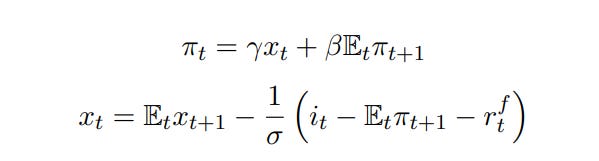
The New Keynesian model starts by adding in monopolistic competition, which will distort the level of output, and adds in sticky prices. The most analytically convenient form of this is to say that a random portion of firms 0 to 1 are able to change their price in each period. (We say that they are visited by the Calvo Fairy, after the inventor of this trick). Now, prices and money matter. If the central bank should cause there to be an unexpectedly high price level, then not all of the firms can adjust their prices to the new equilibrium. We will have rising output. Conversely, a price level too low would lower output. We can think of this as supply and demand curves, like in regular microeconomics. These are the first two equations in the three equation New Keynesian model.

This better matches the facts. We are extremely sure that money has real effects, and that consumers cannot see through the central bank’s policy, although in the long run they will anticipate the central bank’s actions and they cannot be consistently fooled. (A good piece of evidence for this is Coglianese, Olsson, and Patterson (2024), who use the Riksbank in Sweden hiking interest rates for essentially no reason at all. There was a reduction in employment over the next two years, driven by the sectors with the stickiest wages. Similarly, Fukui, Nakamura and Steinsson (2025) find that differences in central bank policy – specifically, whether they peg their currency to the dollar so that it trades at a fixed rate, or let it float – lead to frankly enormous differences in GDP over time).

The first equation governs the supply side, and the second equation governs the demand side. We can thus think of this as our ever familiar supply and demand graph, with the vertical line being long-run supply.

The central bank influences households through its choice of interest rate. While we have excluded capital for simplicity, households are still able to save by purchasing government bonds, which pay interest. If the interest rate rises relative to consumers beliefs about what inflation will be, then consumers will pull their money out of present consumption and put it into bonds. The opposite prevails when the central bank lowers interest rates. If the central bank sets a constant interest rate, then the resulting rate of inflation is in fact indeterminate – any level of inflation is supportable with any level of interest rate. Thus we close the model with a third equation describing how the central bank reacts to changes in the rate of inflation, where they raise interest rates by more than the change in household expectations. This is conventionally called the Taylor Rule, after John Taylor, and the critique of interest rate targets comes from Sargent and Wallace (1975).

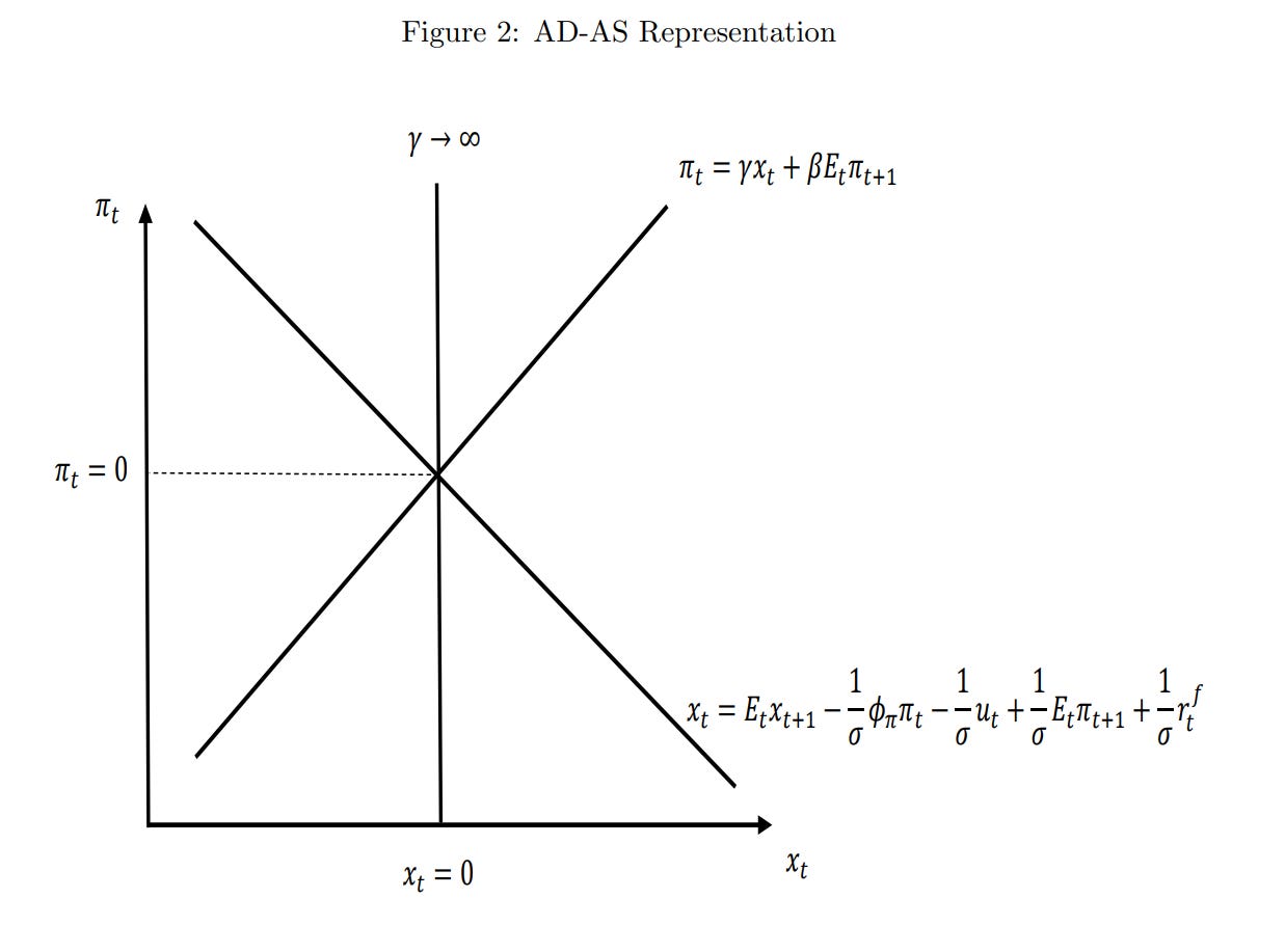
Our optimal policy target, under this model, is to target 0% inflation. This is the Divine Coincidence – it turns out that targeting that uniquely minimizes allocative distortions from firms not being able to change their prices, and also minimizes the shortfall in output. There is no tradeoff between Targeting 0% inflation basically turns the demand curve sideways. Now when there are shocks, nothing happens.

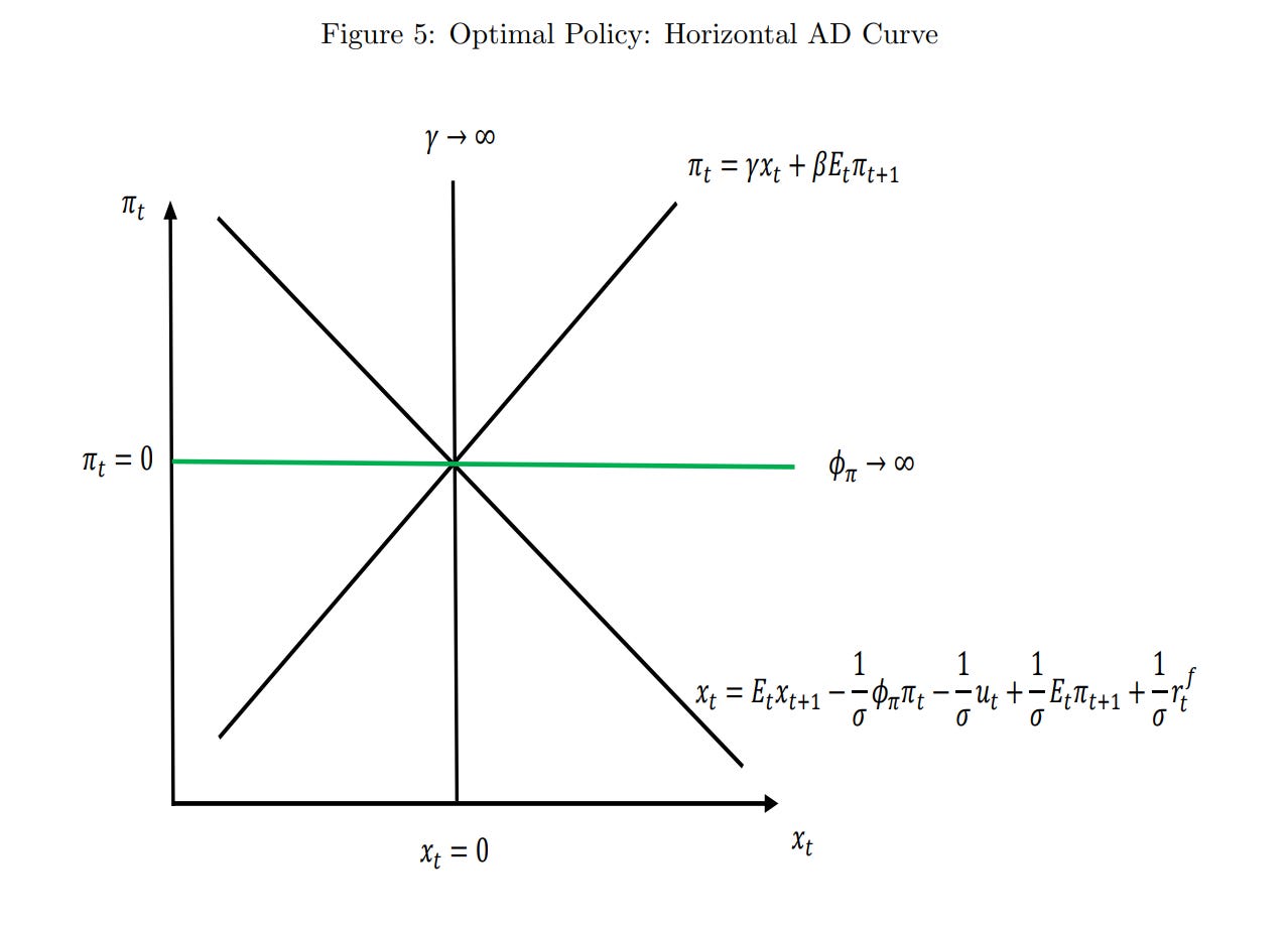
To put it intuitively, (at least, intuitively for me), imagine we start out targeting 0% inflation. A negative productivity shock in part of the economy occurs, and only a fixed percentage of firms are able to change their costs. Some of them won’t, and we will get misallocation from the optimal price. Remember that deadweight loss from a tax increases quadratically as we get away from the optimum point, because it’s the triangle underneath the curve. We would rather share that shock among many sectors, rather than have one sector take on all of it. Lots of little shocks add up to much less than one big shock, when they’re all squared.

Note that there are a lot of really strong assumptions that go into this. We need to assume that the only rigidities are nominal, not real. We need to precisely follow the Taylor rule. Everything in the model has to be linear. Please do not interpret this as an incautious call for a 0% inflation target.

You can extend this to many sectors with different rates of price adjustment, as in Rubbo (2023), where we try to minimize a Consumer Price Index with sectors weighted by frequency of price changes; or we can consider a world where firms actually pay a fixed cost (invariant to the size of the price change) in order to change their prices, as in Caratelli and Halperin (2025). In the latter, we are actually trying to stabilize some aggregate, like wage income; when a shock comes, we now are okay with higher or lower inflation because we don’t want the shock to cause lots of unnecessary price changes in other sectors. Note that NGDP targeting, which you may have heard of, is the latter, with the aggregate we’re stabilizing being the nominal value of economic output.

I would like to emphasize that what we should care about are wages, not prices. (At least, I think!). I was pretty affected by Basil Halperin’s 2021 blog post on the subject. This requires changing our model, because we set it up with sticky prices, not wages. Yes, both are sticky – but they are sticky in different ways, and if we have to pick one, we should pick the one which causes much bigger distortions. Wages are sticky in a way that fits the basic story of Calvo pricing, while prices are closer to the fixed-cost-of-changing-prices story. The way you can tell them apart is to look at the way in which prices change during periods of higher inflation – if Calvo pricing, then the price changes should become larger, and if menu costs, then the price changes should become more frequent. Dvorkin and Marks (2024) found that wage changes did become more frequent during the Covid era inflation. Meanwhile, Nakamura, Steinsson, Sun and Villar (2018) found in the goods market that higher inflation results in no change in the absolute size of price changes, only an increase in their frequency.

My intuition is that wages are more important. If only some products can adjust their prices, that’s okay, because there are lots and lots of different products. You should be more able to easily substitute from one good to another. On the other hand, your wages not changing mean that you must cut back on absolutely everything. This is surely much more important. I do not, however, have a formal proof of this, and the preceding comment should be seen purely as obiter dicta.

Given that a 0% inflation starting point is optimal in either framework, why is it the case that we target 2% inflation instead? The basic argument for it is that wages are asymmetrically sticky, and basically never fall within a job. (They may fall from job to job, but one never gets an explicit pay cut). There is, to my mind, ample evidence that this is the case from microdata on workers. Grigsby, Hurst, and Yildirmaz (2019) have data from ADP, a payroll processing company, and find that only 2% of job-stayers receive a pay reduction in any given year. Hazell and Taska (2024) have data from Burning Glass, now Lightcast, which has extensive data on employment listings – they find that, not only do people on the job not change, new hires don’t change either. (Later work by Hazell, Patterson, Sarsons, and Taska (2022) would document extensive uniform pricing of wages across regions which differ substantially in labor demand and supply – there’s a lot of room for heuristic pricing in the labor market). If we grant this, then we would want a gentle inflation to allow firms to “cut” wages by simply holding them fixed in nominal terms.

I don’t think why wages are sticky downwards is really all that necessary to answer, as we know they pretty consistently are; nevertheless, the standard explanation is that business owners believe that cutting wages will lower morale, as Truman Bewley (1999) found when simply asked a lot of business managers why wages don’t fall during a recession. (Truman Bewley, incidentally, is behind one of the earliest models tackling heterogeneity). This hardly explains why wages are sticky for the new hires, as in Hazell and Taska (2024), though.

At risk of a too long digression, I have a theory of my own: both workers and firms sign long term contracts, but then face uncertainty over how much the products they produce will be demanded. For that reason, firms have flexibility over hiring and firing. They don’t have flexibility over wages, however, because the firm would always like to pay its workers less for the same work. If they face an adverse demand shock, then it would be incentive-compatible to let workers go or to reduce their hours; if they do not have an adverse demand shock, they do not gain anything at all from laying off workers.

Note that these aggregate demand shocks (the money supply equals aggregate demand) must be unanticipated. If they are anticipated, then we will simply raise prices without changing output. Basically the Calvo fairy is not a deep parameter, but rather varies depending on the circumstances.

So far we have been treating agents as identical. We say that there is a representative household, whose characteristics are the average of observed people in the economy. Calculating the impact of a change in monetary policy is then extremely simple – just solve for what the household would do, and multiply by by the population. If you try to set up the problem of the economy as a game with distinct agents, where the decisions of households affect the payoffs of other households, you will very quickly become totally uncomputable. The number of possible paths to solve for increases as an exponent of the number of agents. I am pretty sure that if you tried to solve such an agent-based model without extreme simplifications on their decision making process for the entire United States, you would not be able to finish calculating it before the extinction of the solar system.

The first step toward tractably dealing with heterogeneity was to have a two agent model, or TANK. You have one agent who has a higher net worth, and thus is insured from shocks, and another agent who has a lower net worth and is thus hand to mouth. These two agents will differ in their marginal propensities to consume, which may be due to their inability to fully insure their risk.

HANK allows for more detail in the distribution of propensities to consume, in order to match the empirical data. To get around the computational problems, we do not consider the people as individual agents, but simply as a continuum of types. I do not profess to entirely understand what is going on under the hood, but recent work such as Boppart, Krusell and Mitman (2018) and then Auclert, Bardoczy, Rognlie, and Straub (2021) gave us algorithms for speeding up solving the model by about a factor of 300. (And their model takes 12 hours to solve normally!!) Obviously, this made using it impossible beforehand.

Much of the work has been on trying to understand how monetary policy is transmitted to the economy. I draw mainly from “Monetary Policy According to HANK” by Kaplan, Moll, and Violante (2018) here, as well as “Fiscal and Monetary Policy with Heterogeneous Agents” by Auclert, Rognlie, and Straub (2025). In the representative agent paradigm, the effect of monetary policy works exclusively through intertemporal substitution – facing higher interest rates, households save more now, and facing lower interest rates they spend more now. The consumer is trying to equalize utility in all periods, and so cares only about their permanent income. Transitory shocks don’t really matter. In fact, in RANK models a condition called “Ricardian Equivalence” can often prevail, where deficit spending has no impact on present consumption at all. Consumers anticipate future taxes to pay off the debt, and save exactly enough to offset the present effect on spending.

In HANK, however, fiscal transfers funded by debt matter, and will continue to matter after the transfers stop, which better fits the fact. There will continue to be multipliers over time. This is a big advantage of the HANK approach, and is a much cleaner way to match observed facts than other models. In fact, it’s conceivably possible for fiscal stimulus to pay for itself. (Shush shush though! Don’t say it too loud, some people will get the wrong idea). Debt-funded transfers will, however, increase inequality in the long-run. Since higher income households save more, they will consume less now and consume much more in the future.

The path of transmission is substantially different with heterogenous agents. This is emphasized by Kaplan, Moll, and Violante. In RANK, everything is happening through intertemporal substitution, but micro studies on that have always found too little of this to explain observed macro responses. Instead, what’s going on is that the effect is largely indirect, through a small change in intertemporal consumption spilling over into the real economy.

Since the way in which monetary policy affects the economy needs to pass through indirect channels, they can no longer be so divorced from the structure of the economy created by the fiscal authority. Choosing whether to consume now or later is much cleaner, much more agnostic to the nature of the economy than when some goods are bought on credit and some aren’t, for instance. A more flexible labor market would imply that the effects of stimulus are larger, because people would be able to find additional income to satisfy their desire for goods now. They didn’t need to seek income before, because you had access to credit and could just borrow.

In HANK, neither the aggregate effects of monetary policy, nor its distributional effects, are neutral anymore. The effects of policy will depend sharply on who it affects and in what way. A government stimulus program which targets lower income people will have a greater effect per dollar than one which targets everyone equally. Cash transfers will have a bigger impact than tax cuts, given the current system.

A related line of literature, though not commonly thought of this way, is that the way in which transfers are labeled or thought of has extremely real effects. “Mental accounting”, where people designate some funds for different things and adjust their spending within a category of goods rather than across their whole budget when they get an unexpected windfall, is extremely real. Hastings and Shapiro have several papers on this – in one, when gas prices change, people switch between premium and regular gasoline in ways that are inconsistent with them treating “gas money” as something that can be put to other uses. They then show that food stamps lead to an increase in the amount spent on food, even though it should surely lead to them redirecting what they were spending on food to other tasks just like it were income. Boehm, Fize, and Jaravel (2025) showed, from an experiment in France, that having the cards with which transfers were made expire substantially increased consumption after getting the transfer, when, again, it should be fungible with cash.

The structure of debt now matters, as well as the way in which interest rates are manipulated. A natural starting point for models is that debt rolls over every period. Changing this actually does affect monetary policy – the longer the duration of debt, the less the effect of monetary policy. This all ties back to the imperfect consumption smoothing that is at the core of HANK. Similarly, while in RANK a series of small changes in interest rates can add up to one large change, in HANK you would be better served doing it all in one go. Doing it up front allows more time for the change to amplify itself.

It’s not really a prediction, but I do appreciate how it provides a microfoundation for the “long and variable lags” which have bedeviled macroeconomists. If things are only happening through changes in people’s actual behavior, that takes time to kick in.

So, those are all the ways in which HANK delivers different predictions than RANK in how the structure of monetary policy differs. However, it is not at all clear that HANK delivers different aggregate predictions from a RANK model. Without those differences in aggregates, there is no amplification.

There are two fantastic papers out recently, “The Matching Multiplier and the Amplification of Recessions” (2023) by Christina Patterson, and “HANKSSON” (2025) by Bilbiie, Galaasen, Guerkaynak, Maehlum, and Molnar, showing why this matters. They want to greatly simplify HANK to the minimum number of statistics sufficient to find the whole effect of aggregate demand shocks, which are two.

The first is how much different the aggregate marginal propensity to consume (MPC) is from the average MPC. If everyone has the same elasticity of income with respect to an aggregate demand shock, then the average and aggregate will be the same. If, on the other hand, higher MPC individuals have a different elasticity of income when a shock comes than lower MPC individuals, the aggregate demand shock is either amplified or dampened. Put concretely, if there’s a negative aggregate demand shock, and the people who lose their jobs first are those who spent the greatest portion of their paycheck, the aggregate demand shock is amplified.

This is what Christina Patterson does for the United States. She uses income data from the PSID to estimate marginal propensities to consume for very detailed demographic characteristics, then uses that to impute MPCs for data on firm-employee payments with the LEHD. She finds that higher MPC workers are more exposed to recessionary downturns – which, to be fair, is hardly surprising. We have long known that the lower-income workers get fired first, which can have such an effect that the measured wages of those who are employed can actually rise during recessions purely through changes in composition.

Patterson’s paper is very good, but does not fully identify the effects without an assumption of constant saving behavior. HANKSSON, which is an acronym standing for “Heterogenous Agent New Keynesian Sufficient Statistics Out of Norway” goes one step beyond by just getting the actual consumption and saving behavior of every single person in Norway. (What!?!? Yes!). They have the complete personal consumption behavior of every single person in Norway from 2006-2018. I am frankly flabbergasted that this exists, and I’m sorry for hanging on this point for a while, but holy cow this is an incredible dataset.

Anyway, in HANKSSON, they find that there is at most a negligible difference between the average and the aggregate MPC. Thus, a model with representative agents may be wrong about how the shock happens, but it is right on the aggregate predictions. Their model allows them to evaluate counterfactuals with different tax and transfer systems, in particular that of the United States. Importantly, the lack of aggregate heterogeneity is not a function of the more extensive system of welfare in Norway than in the United States. While this does not rule out cultural differences, it’s pretty powerful evidence that heterogeneity may not matter, for now.

I see this as being effectively a return to the simple two-agent models. There, there are two groups of people, one liquidity constrained and the other not. The elasticity of consumption with respect to aggregate demand shocks must average 1 across the two groups, so if they’re both 1, then it’s RANK. Otherwise, you’ve introduced the object which Patterson and Bilbiie et al are studying.

There has been some criticism of HANK on the grounds that it simply isn’t necessary. Debortoli and Gali (2024), for instance, argue that two agent New Keynesian (TANK) can approximate whatever HANK can do. However, I found Matthew Rognlie’s comments on the paper convincing. Fundamentally, HANK is closer to reality. You need a reason to move away from it. For Debortoli and Gali, that reason is tractability – but if modern methods make richer heterogeneity tractable, then you should simply use that. Also, the claim that TANK could approximate HANK is dependent upon there not being a persistent rise in marginal propensity to consume, but as Rognlie points out, the studies they rely on to show this do not rule out a persistent rise, but are simply insufficiently powered to detect it.

There is even a case to be made that monetary policy, in spite of everything which has been said up to this point, is the wrong laboratory to think about the importance of heterogeneity on aggregate demand. Go back to proposition 2 of Auclert, Rognlie, Straub (2024). Suppose that the government will hold no debt in the steady state, meaning that they will pay back their debts with tax revenue. For any given interest rate shock, HANK and RANK will give you the same predictions. Heterogeneity will amplify the effects, but the high MPC agents will be less sensitive to that change in interest rates. The two will exactly balance each other out. It is every other kind of shock which will have very different impacts, and only the interest rate shocks which will have this equivalence result. So, HANKSSON does not show that there is no aggregate importance

So what have we learned from HANK? I think it has emphasized that the distributional consequences of monetary and fiscal policy do really matter. I also think that aiming toward realism in a model is good – we cannot rely upon the equivalence of RANK and HANK. We don’t have enough iterations to reasonably take Friedman’s dictum that it is only the predictive power of a model that matters. To quote Kaplan, Moll, and Violante,

“Taking a broader perspective, there are additional reasons why it is important to develop a full grasp of the monetary transmission. First, as economists, we strive to gather well-identified and convincing empirical evidence on all the policy experiments we contemplate. However, this is not always feasible, as demonstrated by the recent experience of central banks that were forced to deal with a binding zero lower bound by turning to previously unused policy instruments. In these circumstances, well-specified structural models are especially useful to extrapolate from the evidence we already have.

Moreover, the relative size of direct versus indirect effects determines the extent to which central banks can precisely target the expansionary impact of their interventions. When direct effects are dominant, as in a RANK model, for the monetary authority to boost aggregate consumption it is sufficient to influence real rates: intertemporal substitution then ensures that expenditures will respond. In a HANK model, instead, the monetary authority must rely on equilibrium feedbacks that boost household income in order to influence aggregate consumption. Reliance on these indirect channels means that the overall effect of monetary policy may be more difficult to fine-tune by manipulating the nominal rate. The precise functioning of complex institutions, such as labor and financial markets, and the degree of coordination with the fiscal authority play an essential role in mediating the way that monetary interventions affect the macroeconomy.”

You also need HANK if you place different weights on different people, or do not only care about aggregate impact but also how it is allocated. This could be as simple as declining marginal utility as a function of wealth, which is the usual justification for redistribution. Nothing else can do this quite right.

The biggest policy-relevant thing that HANK teaches us with regard to monetary policy is that changes in monetary policy will have persistent effects on outcomes. This is quite relevant for the post-COVID period. It is not enough to observe that the fiscal and monetary stimulus had such and such an impact on outcomes, and to assume that that is that. Changes in the distribution of consumers by wealth will continue to have an effect on the distribution of consumers. The long and variable lags of Friedman are very real.

Oddly enough, I see much of the point of HANK applying to fiscal shocks, not monetary ones. The central bank does not have unlimited powers, because their interest rate changes will affect the real cost which the government spends on servicing debt. Poorly conceived or ill-designed fiscal schemes may land us in a sticky spot, like it did after COVID.

One hopes that it will inform our forecasting in the central banks for the better. This is entirely too early to tell, however – central banks have to be institutionally conservative, and the first tries at using HANK for forecasting had poor results. I will pass on speculating here.