An Introduction to Auctions

How much can we trust the empirical auction literature?

The goal of economics is to possess sufficient knowledge of the underlying causes of behavior so as to make predictions about the future. To do this, we write down a model explaining how we think a thing caused another thing, and then we find the appropriate values to plug into it. The latter step is not trivial, and it is for that purpose that we have developed the whole econometric toolkit, as I have previously discussed on my blog.

Either of these steps going wrong, though, is sufficient for our predictions to be inaccurate. It is possible that our numbers are wrong, in which case the model might be said to be misidentified. It might also be the case that our model of how data is generated is wrong, in which case we might say that it is misspecified.

One laboratory in which economists work is auctions. Hundreds of billions of dollars worth of goods and services change hands in auctions every year. These markets diverge from the idealized frameworks enough that their design really matters, and economists have put considerable work into making them better. One of the great successes of economists was the auctioning off of radio spectrum frequencies in the 1990s, which generated billions of dollars in surplus. I am writing this to explain all that we know, and to celebrate what is possible.

I am also writing this essay to caution. We have both made incredible progress in estimating the parameters of auctions, and yet have so far to go. We know much less than we think we do about auctions. The assumptions needed to uncover the distribution of valuations are restrictive, and often not met in practice. These assumptions are not trivial, and often suffice to flip the sign of the results. I very often see papers make assumptions, often in a throwaway tone, which are wholly responsible for the observed results. This is not a field which you can very well venture into, reading only the abstracts and expecting never to be misled. One must, in order to choose to believe these papers, carefully consider how their assumptions interact with the results which they have found.

The area which this essay could traverse is enormous. Many things will be omitted entirely, and readers interested in a more comprehensive coverage for empirical auction estimation should consult Hortascu and Perrigne (2023). In particular, I am leaving a section I had begun writing on the estimation of online auctions such as eBay for a later article. We will also be glossing over scale auctions, multi-unit auctions, and auctions which are part of a dynamic discrete game.

Instead, we will cover the basic facts of auction theory, and show how the idealized predictions can break down. We will then discuss estimation of the underlying valuations of the bidders which allow us to make counterfactual predictions, and discuss the assumptions we must make. We will then cover how we can make do, even with unrealistic assumptions, and we conclude with recommendations for future research.

i. Theory

Let’s start by establishing some facts and definitions. The auction you are likely most familiar with, where there is an auctioneer calling out bids, is called an English auction. In that, the bidding continues until only one bidder remains, and then the good is sold at that price. It has its companion in the Dutch auction, which goes in the opposite direction. The price is set above anything anyone would be willing to pay, and then lowered. The first person to buzz in buys it at the price that prevailed when the countdown stopped. These are also referred to as ascending and descending auctions.

Those auctions take place over time. We could compress it to one round, and have a sealed bid auction, of which there are two forms: first-price and second-price. First-price is the more intuitive of the two. Everyone submits a bid. The highest bidder pays the price they submit. A second-price auction has everyone submit a bid, and then the highest bidder buys the good, paying the second highest price. Why would any auctioneer do this?

In theory, the revenue obtained is not any different. If everyone is drawing from the same distribution, bidders are risk-neutral, everyone’s value is uncorrelated, there is no collusion, and the number of bidders is known, the auctions will give us the same revenue. This is called the Revenue-Equivalence Theorem, and was established by Roger Myerson (1981). In the first price auction, everyone shades down their bid so as to maximize their expected payoff. This is easily calculable given your own valuation, since you know the likelihood that you are the highest bidder, and the expected value of the next highest bid. Everyone bids the price that the next highest bidder would have bid at, and thus the second and first price auctions converge to the same outcomes.

The second-price auction has the great advantage that there is no incentive to misreport your valuation. Think through it. Suppose you lower your bid below your own valuation. This will not change the price you pay for the good, unless you lower it so far that you do not get the good at all. Underreporting is never profitable. If you are the highest bidder, overreporting does not change the price you pay. If you are the second highest bidder, reporting above your valuation only wins you the good when your value is less than what you paid for it. Therefore, overreporting never increases your pay-off either.

What’s more, the English and the second-price auction, and the Dutch and the first-price auction, are in fact the same thing. In the ascending auction, the price increases until all but one drops out, and then the good is immediately sold. There is no incentive for you to misreport your values for the same reason that there is no reason to continue bidding while you are ahead. Likewise, in a Dutch auction, the winner pays what they bid, and are thus incentivized to shade down their bid, by waiting a bit longer before pressing the button.

With independent private valuations and no entry costs, there must exist a reserve price which will raise revenue for the seller.

Suppose that we have 2 bidders, who have values drawn at random from the domain [0,1]. We will have a standard second price auction, and the expected value is ⅓, because the formula for the outcome of a second price auction under those circumstances is (n-1)/(n+1), where N is the number of bidders. The optimal reserve price is .5. Half the time, that is the price; a quarter of the time, both bids are above with an expected value of .66, and another quarter of the time the good isn’t sold. The expected revenue would be 5/12ths, which is clearly better.

ii. Breaking Equivalence

Now, don’t take the revenue-equivalence theorem too strongly. In practice, the form of the auction matters. As noted above, everyone must be drawing from the same distribution, bidders must be risk-neutral, everyone’s value must be uncorrelated, there must be no collusion, and the number of bidders must be known for it to hold. Knowing this is as result is an excellent starting point, though, because it allows you to isolate what exactly you are breaking, and thus what to fix.

One of the most common ways for revenue to break down is if values are correlated with each other. Rather than everyone drawing a private value, they instead receive signals of the good’s value drawn from some distribution. If you naively bid the value of the signal, you will win if and only if the signal you received was higher than everyone else. You wouldn’t ever want to win such an auction. If you have beliefs about the distribution, then you can shade down your bid, but auctions in which people can learn something about the bidders, like an English auction, will come to different results than those which occur simultaneously. If everyone’s valuation, in a perfect information world, is the same, then the auction is said to be a common value auction.

Common value auctions reverse much of our intuitions when it comes to outcomes. Take what happens when we add in risk aversion. If values are common, then risk aversion will reduce revenues for the seller, and more competition will actually reduce the profits which they get. Remember that while everyone shares the value, they receive signals about that value drawn from some distribution. The average value of that distribution is accurate, but simply bidding your valuation would be “wrong”, and lose you money. Since these losses are particularly painful when you are risk averse, you shade your bid down by even more.

However, with independent values, risk aversion actually increases the revenue for the seller in a first price auction. This is a bit less intuitive, but essentially the bidder wants to minimize their variance in the utility received. When a bidder shades their bid by more, they are increasing the likelihood that they are either get a lot of profit, or none at all. A risk averse bidder is willing to take the lower expected value for higher certainty.

Or take adding in another bidder, especially with risk aversion. If values are independent, adding in another bidder must increase the revenue for the seller. You’re just taking another draw from the distribution. With a common value, it will instead keep revenue the same (if people are risk-neutral) or reduce revenue if bidders are risk-averse.

Private information will break revenue equivalence, because it creates heterogeneity in the bidders. An example of this in practice would be a tract of land being auctioned off for offshore oil drilling, as in Hendricks and Porter (1987). Some of these tracts abut other tracts which have already been drilled, while others are away from anything else (and called “wildcat” tracts). Everyone has the same information about wildcat tracts, but drilling companies possess private information about the tracts that abut their land. They might know that the oil field they are drilling is to the South and East, and stops partway through their land. They will call for an auction on all of the plots of land surrounding their track, but will only bid on the more valuable plots to the South and East. Anyone who wins a plot to the North will be left with a worthless swathe of ocean, while the incumbent can get valuable land on the cheap. Note that the auction will not collapse into the incumbents getting it for free – the incumbents must bid enough such that expected profits for entrants are zero – but they will get it at a considerable discount. Hendricks and Porter show that, while oil is much more likely to be found on adjacent tracts, these tracts see fewer bidders and higher profits for the incumbent.

The presence of entry costs also flips our intuition. With no entry costs and independent private values, having an additional symmetric bidder is always good. In fact, it’s always better to have one more bidder than to set a reserve price, as shown by Bulow and Klemperer (1996). Remember that the reserve price is essentially entering your own auction as a bidder, and sometimes you will “win” and be unable to sell the good. Obviously, you would prefer a bidder with the same expected value who can actually win.

Suppose though, that we have entry costs of the following form: prospective bidders know the distribution from which their valuation will be drawn, but have to pay a cost to find it. This is akin to a firm paying someone to evaluate whether items are worth buying. Suppose that there are enough bidders that you wouldn’t want to enter every auction – if you did, the likelihood of you winning would be too low to sustain the fixed costs. In that case, bidders will randomize whether they enter or do not enter the auction. (Since all the bidders are assumed to be symmetric, their strategy will all be the same).

When firms randomize entry, though, sometimes you get lots of bidders and sometimes you get very few. These cases are not symmetric. The marginal value of an additional bidder gets increasingly smaller. You’d far rather the same number in each auction. Thus, Levin and Smith (1994) show that with entry costs the seller will actually profit by restricting the number of allowed bidders to a pool, such that the optimal strategy is to always enter. If unable to restrict the number of bidders, then the seller should sequentially offer the right to enter. If bidders have some signal over their valuation, as in Roberts and Sweeting (2013), a sequential negotiation mechanism can actually be optimal.

iii. Estimation

Thus far, explicitly or implicitly, we have been focusing on how someone can design a mechanism. What we can also do is use the auction to infer how much customers value a good, and thus, demand curves. So long as the number of bidders is known, you can use observed bids – or even just the winning bids – to infer the entire distribution of valuations for a good, without making any assumptions at all about how those valuations are distributed.

In order to make these claims, however, we must make assumptions about the nature of buyers, assumptions which I believe do not hold up in practice. We must make some claims about the homogeneity of the bidders, about the risk aversion of the buyers, of how entry works into the auction, of whether valuations are independent of each other and of your prior valuations, and about what other bidders know about the auction going in. There is good news and bad news.

That the distribution is identified with infinite data and independent private values is easiest to see with second-price auctions. Here, we are just asking people to report their valuation, so they will honestly report it. If you see all of the bids, then you can just draw a histogram of their valuations, and that is your distribution. (Strictly speaking, you don’t even need the number of bidders for this). If you possess only the winning bids, then you know what the likelihood of that bid being the number one bid given an arbitrary cumulative density function, and with the number of bidders, you can trace out what the whole system is. In fact, so long as the position of the bid is constant, you identify with any of the bids – only third place, only fourth place, only fifth place, and so on.

You can also do this for first price auctions, so long as the number of bidders is known and firms are symmetric, starting with Guerre, Perrigne, and Vuong (2000). Start out with observing all of the bids in a first price auction. We assume that all bidders are symmetric, meaning (in practice) that they share the same distribution, which they know, but we do not. They receive a new valuation from that distribution in each auction, and there is no correlation from round to round (as allowing for that would introduce strategic considerations likely making it impossible to solve).

We start by putting a kernel density function around each of the data points. The point of this is to smooth out the data, like a histogram. Then, given this distribution of bids, we can estimate their cumulative distribution function, and estimate how much firms would mark down their bids, given what we know about the bid distribution. What makes it work is that since the bids are monotonically increasing in the underlying valuation, we can invert the bidder’s optimization problem and solve.

Prior work on estimating auctions made what are called “parametric” assumptions, where we assume that the distribution of valuations followed some standard form. A normal distribution is a type of parametric distribution, for example. GPV do what is called “nonparametric” estimation, where we make no assumption whatsoever about the shape which the distribution of values should take. GPV’s method is actually much more easy to compute than parametric estimation, contrary to what I expected (where parametric assumptions are often used in order to simplify the space of possibilities). Since we have an equation to solve for, we can just plug in the numbers and call it a day. Parametric estimation doesn’t have a clean solution, so we have to essentially guess-and-check a series of parameters.

My biggest concern with the auction literature is that the models are misspecified, and misspecified approximately all of the time. In order to make estimation tractable, we have to make lots of assumptions, which are absolutely not trivial assumptions to make. The assumption of independent private values in Guerre, Perrigne, and Vuong is loadbearing. If valuations are correlated at all, the identification breaks down.

Now I want to discuss some examples of auction estimation in practice, and illustrate how they deal with the limitations of the data. I am going to be taking a high level gloss on these papers, so if you want to work through the models yourself you will need to turn to the paper. Athey and Haile (2002) is an important formal guide to when an auction is identified – in general, you cannot have the anonymity of GPV, but need information on the identify of the bidders, or plausibly exogenous shifters in the number of bidders or the form of the auction. For common values, you do not so much identify the valuations, but compare predictions using the exogenous shifters.

iv. Auction Estimation In Practice

The selection of papers here is by necessity idiosyncratic – reading everything would take weeks. I will try and highlight how confident I am in each of them – please do not take its inclusion as an uncritical endorsement.

This paper is one I quite like. Athey, Levin, and Seira (2011) have data on forestry auctions, which has been a market well-traversed by economists. Much of the land in the American West is publicly owned, so the right to use tracts of it is sold at auction. The Forest Service would announce that an auction was to be held, and offer a “cruise” around the area, to allow potential buyers to evaluate the quality of the forest cover and the difficulty of extraction. There were two kinds of buyers, mills and loggers. Mills owned their own processing equipment, and so tended to have higher valuations than the loggers, who were smaller. The authors make the assumption that the values of the mills are such that the top two mills beat the highest value of the loggers. The model is considerably simplified – and matches the data better – by doing this, as we only need to concern ourselves with the entry decisions of the loggers.

These auctions were, importantly, conducted in two different ways – open outcry ascending auctions (gimme 15, I have 15, gimme 20, gimme 20, sold!) and sealed bid first price auctions. The form of the auction was determined, in many cases, entirely at random, which will be important for finding their results later.

Their model allows for there to be costs to enter and that there are independent private values condition, with no risk aversion or common values. This would seem shocking, because surely there is a substantial common value component to the plot of land. Even if the common value component of the amount of accessible board-feet on the tract were known with certainty (remember that the common value component is important only insofar as it is observed with error), the bidders will be affected by the same common shocks to the value of timber.

It is the randomization of open versus sealed-bid which allows them to tell the two apart. If there were a substantial common value component, then it implies that one should see higher bids in open outcry than in sealed-bid, but it is in fact the opposite. What is going on instead is collusion. In the open auctions, it is extremely easy to collude and impossible to defect. If you try and bid above where you promised you would bid, the auction simply continues, and you get nothing. Only in sealed-bidding is defection possible, and so sealed-bid auctions reduce collusion and give loggers a chance.

With the model, they estimate the parameters and find that the sealed-bid auction is more efficient. This is a bit of a surprise, because the open outcry auctions, even with collusion, will always allocate the good to the right company. In any case, though, the differences in social welfare are small, and the forest service auctions were reasonably close to optimal.

Yunmi Kong (2020) has a paper on bidding for tracts of land in the Permian Basin for drilling oil wells. It’s a paper which is made, in truth, by Figure 3, which shows the price paid for land at open (O) and sealed (S) auctions, normalized so that the bottom is the reserve price.

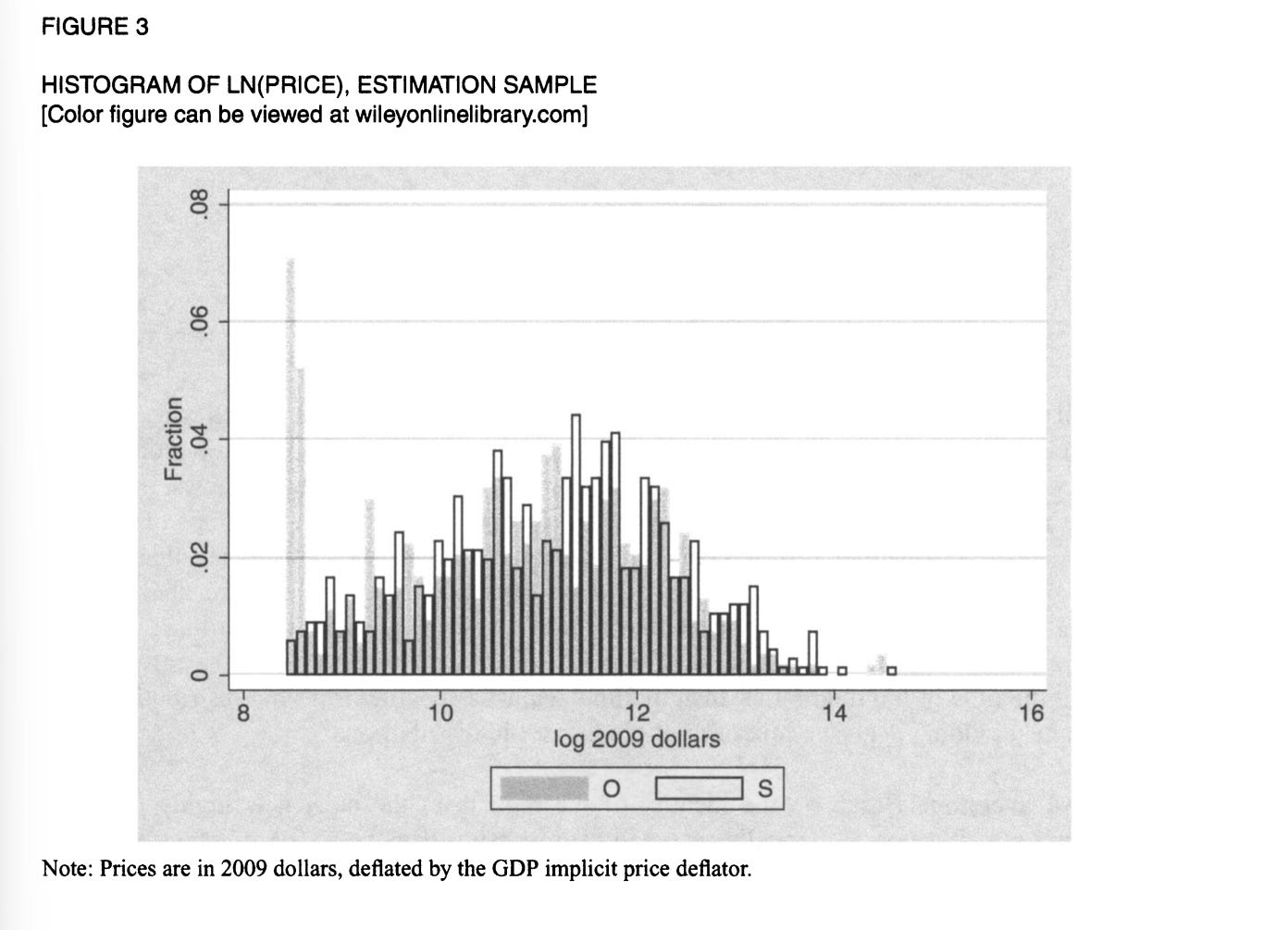
As you can see, there is an extraordinary heaping of prices at the reserve price for the plots of land for open outcry auctions, but not for sealed bids. When bidders turn up, and see they’re the only ones there, they bid the minimum. To explain why people aren’t bidding the minimum in sealed bids, he claims that bidders are quite risk-averse. By implication, this means that it is private values which dominate, because if you’ll recall from earlier, leads to higher prices in first price sealed bid auctions. He justifies no common values assumption on the grounds that the area has been well-canvassed by seismic surveys, and thus there is no heterogeneity in the signals that bidders receive.

The next is a paper which I am not confident in. Hong and Shum (2002) use data from the New Jersey Department of Transportation to assess the effect of additional bidding competition in procurement auctions. Specifically, they have the bids and the number of bidders, and do not observe the estimated cost of the project or any information about the particular firms. So what do they do to identify the model?

First, they make an assumption that firms are symmetrical. They are unable to take advantage of knowing the identity of firms across many auctions because they not observe the size of a project, although they can categorize it by type. They then break the freedom of non-parametric estimation, and try to estimate the joint distribution of signals and private values. The cost to each contractor is the product of the common value component v, and a private value component a. They assume that the values are drawn from a log-normal distribution, which allows us to say that the standard deviation of each part tells us its relative importance.

From there, they try what happens when there are different numbers of bidders. There is no exogenous variation, nor can they even try and control for the size of the projects. It would seem plausible that larger and more firms bid on larger contracts – there is no attempt to estimate the entry costs that would make that sensible.

Someone who is on the right path, though I’m not convinced of the paper as it stands, is Lindsey Currier (2025). She has a much better data set, covering 1.3 million bids and the whole nation. Her exogenous variation is when a company established out of state enters a different state. When they do so, they faced a substantial cost to become accredited, so they tend to enter lots of auctions at the same time. When new firms enter the auction, the prices paid by the government end up falling, and substantially so.

There is also an assumption of no common value component, which she justifies first on the basis of their being little renegotiation afterwards. This might indicate that contractors were well-apprised of the value, but I don’t buy it. We would expect these firms, who are often not corporations, to be risk-averse. (I will deal with how risk-averse in a future article, as it is a topic which I have wondered about for years, and only now feel like I know enough to answer). Not having to renegotiate is perfectly consistent with them shading their bids!

The other justification is that the effect of plausibly exogenous entry into the market reduces the price paid, akin to how Athey, Levin, and Seira justified the no common values assumption in their paper. This instrumental variable approach to bidder entry is a descendant of Haile, Hong, and Shum (2003), (which is still somehow unpublished after 22 years).

My concern is that the instrument is not actually exogenous here. Imagine a world in which firms are learning about the true cost of projects over time. A new firm will enter when the market is in error – but wouldn’t the market correct over time to the correct price? Then firms entering would correspond with prices falling, when they were sure to fall anyway.

Another instrument which seems more plausibly exogenous, although it will of course have a smaller first stage effect, are changes in the bonding requirements of contractors. Contractors have to post a fixed amount in most states, and this amount is not adjusted for inflation. It seems like the adjustment of this would be essentially arbitrary. I understand, though, the choices which she made.

In another context, entry into bidding from a move to online bidding in India and Indonesia found an increase in bidders, but no change in costs, although there was an increase in quality and speed of construction (Lewis-Faupel, Neggers, Olken, and Pande, 2016). Of course, I cannot complain about an instrumental variable maybe not being exogenous, and then cite difference-in-differences on a time series. It’s worth considering though.

I will deal with whether, and how much, firms are risk-averse in a later essay, and discuss Bolotnyy and Vasserman (2023) then. I mention it now as an excellent paper, but too far afield of what we have been doing.

A paper which I really like is “Choice by Design” by Sam Altmann, which examines an auction system which allocates food to food banks. Feeding America is the largest food bank network in the United States. Much of what they do is allocate food donations between various food banks, especially when large companies like Walmart wish to donate surplus truck loads of food.

The old system was a sequential negotiation. Each food bank was called up on the phone, and asked if they would take the truckload of food. The ordering in which food banks were approached was determined by an algorithm for how recently they had been offered food, and a measure of local poverty. When they get the call, the food bank has a few hours to accept or decline. If the food bank says yes, the mechanism ends and they pay for shipping. Otherwise, it gets offered to whoever is next in line, until someone takes it, or it is returned to the donor.

The new mechanism replaces this with a twice daily auction. Every food bank receives a virtual currency called “shares”, which are allocated to advantage the food banks with higher local poverty levels. Bidders have access to credit, and are allowed to make negative bids, as happens when the load of food is inconvenient or undesirable. Feeding America does this to ensure that donors trust them to always take a truckload off their hands. Sam Altmann found that the new, choice mechanism so improved the allocation of goods that it was equivalent to a 32% increase in total donations under the old system.

It is instructive to look back to Levin and Smith (1994) and consider why the old system is not efficient. The sequential mechanism becomes optimal when entry costs are high. Here, the system is simple and easy to use, so we would prefer to canvass everyone simultaneously.

What I particularly like about it is how it can argue for being incredibly close to the environment where we can just raise off bids. Valuations are determined by idiosyncratic private demand, and there’s no uncertainty over what you’re getting. Collusion is highly improbable, the number of bidders is pinned down and well-known, heterogeneity due to transport costs is essentially a pure function of distance and so can be controlled for, there’s full information, and the presence of free borrowing means risk-aversion is a non-issue. The only complicated bit is that he doesn’t observe stockpiles, so he has to infer this from a repeated game – but this is the sort of thing which is just assumed away because we would never meet enough of the other conditions which could possibly allow us to answer it. I’m extremely pleased with this paper, and it is deservingly in R&R with Econometrica right now.

v. Summing Up

So what would I like to see in papers? First and foremost, there seems to be an untaken opportunity for merging detailed data on the financials of firms and their subsequent behavior at auction. I think it would be useful to merge the Longitudinal Business Database with arbitrary auctions, in order to sort out heterogeneity in firms. I think Currier’s paper is an excellent example of this.

I think there should be more experimental tests of the effects of changes in auction procedure, especially for the government. The number of times I have seen this have been limited, although I have not truly investigated the online, private auctions where this would surely be most valuable. Work analyzing experiments in the laboratory was done by Bajari and Hortascu (2003), but frankly I find this sort of stuff totally unconvincing. (Like the supposed “proof” of the inverted-U relationship between competition and innovation which had a bunch of Zurich undergrads bidding on pretend projects). David Lucking-Reiley (2006) does a field experiment where he himself is buying and selling Magic: the Gathering cards, but it is limited in what it sets out to do. The best, I think, is Ostrovsky and Schwarz (2023), who consulted with Yahoo in order to place optimal reserve prices on advertisements. Here their assumptions were a log-normal distribution of valuations, and then they simulated draws of parameters to check for accuracy.

Finally, I would like for interested policymakers to understand the assumptions which go into making these papers, and to not take their findings uncritically.