The Unreasonable Effectiveness of Cash Transfers

Local fiscal multipliers and slack!

In Monday’s article, we discussed service-led growth – many developing countries are seeing most of their growth in local services, like shops and restaurants, and not in tradable goods. This should be thought of as a multiplier on growth which is occurring for other reasons, and not truly as a cause of growth in and of itself. As countries grow richer, the people prefer relatively more of the non-tradable goods which can only be offered locally. One only has so much of a desire for more wheat or corn before you’re sick of it, after all. As the demand for the non-tradables increases, producers are able to specialize more and produce them more efficiently.

The striking implication of this is that cash transfers are going to be unreasonably effective. We may not face decreasing marginal returns (as one might expect from the usual declining marginal utility of money) but increasing ones. Simply dropping in more cash to a place is not only going to raise the consumption of the people who get it, but also raise the consumption of their neighbors. This is a big deal, because we might otherwise expect a cash transfer program to create winners and losers. While it raises the consumption of some people, it would also raise the prices of goods in the area, impoverishing others. If utility is non-linear, it could even conceivably lower welfare – perhaps by lowering people below a threshold of nutrition.

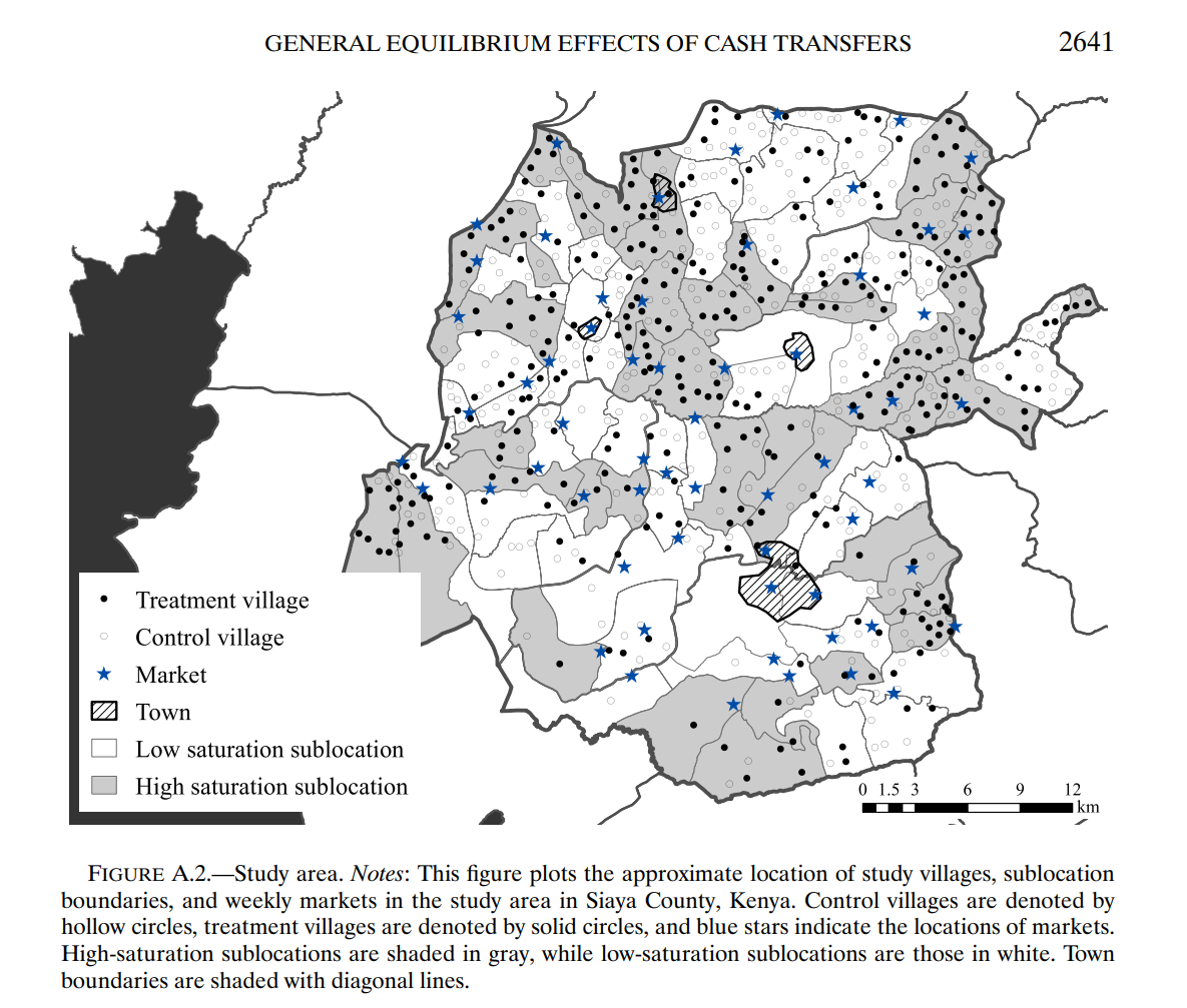
Thankfully, however, the empirical literature disagrees with this, and shows a positive fiscal multiplier. The best study on this is Egger, Haushofer, Miguel, Niehaus, and Walker (2022), who carefully document the effects of an experiment in Kenya. GiveDirectly, a charitable organization of which Niehaus is a founder, allows donors to “give directly” to the poorest people in the world with no strings attached. As you can see below, who received cash transfers was randomized both at the village level, and also into zones where many villages received the cash transfer, and into ones where very few villages did. (Randomization at the village level for a few reasons. One might reasonably be concerned people will share their income with their friends and family, which would break the stable unit treatment value assumption (SUTVA) – if people were very generous, we wouldn’t see any difference in outcomes. Also, as the earlier Miguel and Kremer paper “Worms” showed, you can have direct positive spillovers in other ways. In that paper, some people having their intestinal worms removed meant that they could not then spread it to others, which is another SUTVA violation – you would miss most of the effect, in fact, if you don’t account for this!). In each village, only the poor households – those with thatched roofs – received transfers.

These cash transfers are very large, equivalent to 16% of the GDP in the areas which they treated, or 75% of the average household’s annual expenditure. (The poor countries of the world are very poor, to be clear – this is only a thousand dollars nominal). They collect detailed data on household consumption, enterprises, market prices, and the provision of local public goods, the details of which can be found in section 3. Households that received money immediately drew upon it to buy durable assets, such as livestock, motorcycles, furniture, and farm tools. As you can see, many of these are investments, which ought to go some way in explaining the more muted reaction of enterprise investment.

But that much is obvious. What happens to their neighbors? Their income goes up – by a lot. Annual labor income for non-recipient households increases by $335 PPP adjusted. This is not due to transfers, and can emphatically reject anything more than the most trivial transfers. Rather, it’s all through an increase in labor income. And what happened to prices? At most, the price of goods increased by 1.2%. All told, for every dollar dropped in Kenya, another one and a half dollars worth of consumption spring into existence.

As mentioned earlier, it is possible for aggregate consumption to go up but welfare to go down through price spillovers. Imagine that people have some threshold of nutrition which you need to meet in order to stay alive. Then the experiment might push some underwater, while lifting some people halfway out. Some good news on this, though: we can test for it. Munro, Kuang, and Wager (2025) show that you can get the full effect by finding the elasticities of demand for the goods you care about. Calibrating their results to an experiment in the Philippines by Filmer, Friedman, Kandpal, and Onishi (2023), they find that the welfare effects of the experiment are biased up.

And it’s important to note that Filmer et al has the largest price spillover effects out of all the cash transfer studies. Cunha, De Giorgi, and Jayachandran (2018) report on a Mexican experiment which was a mix of cash and in-kind transfers, and found no substantial price inflation. As a policy question, the effects of cash transfers on prices elsewhere are absolutely not enough to outweigh the positives. Rather, I see Munro, Kuang, and Wager as really about being the sort of data you can collect during an experiment – you can use simple incentivized choice experiments in the course of the regular experiment to get the local price elasticies, and get a complete answer as to welfare.

The papers which I built the earlier blog post off of, Fan-Peters-Zilibotti and Peters-Zhang-Zilibotti, only observe the positive spillovers as an implication of their demand system, and are unable to explain why these increasing returns might exist.

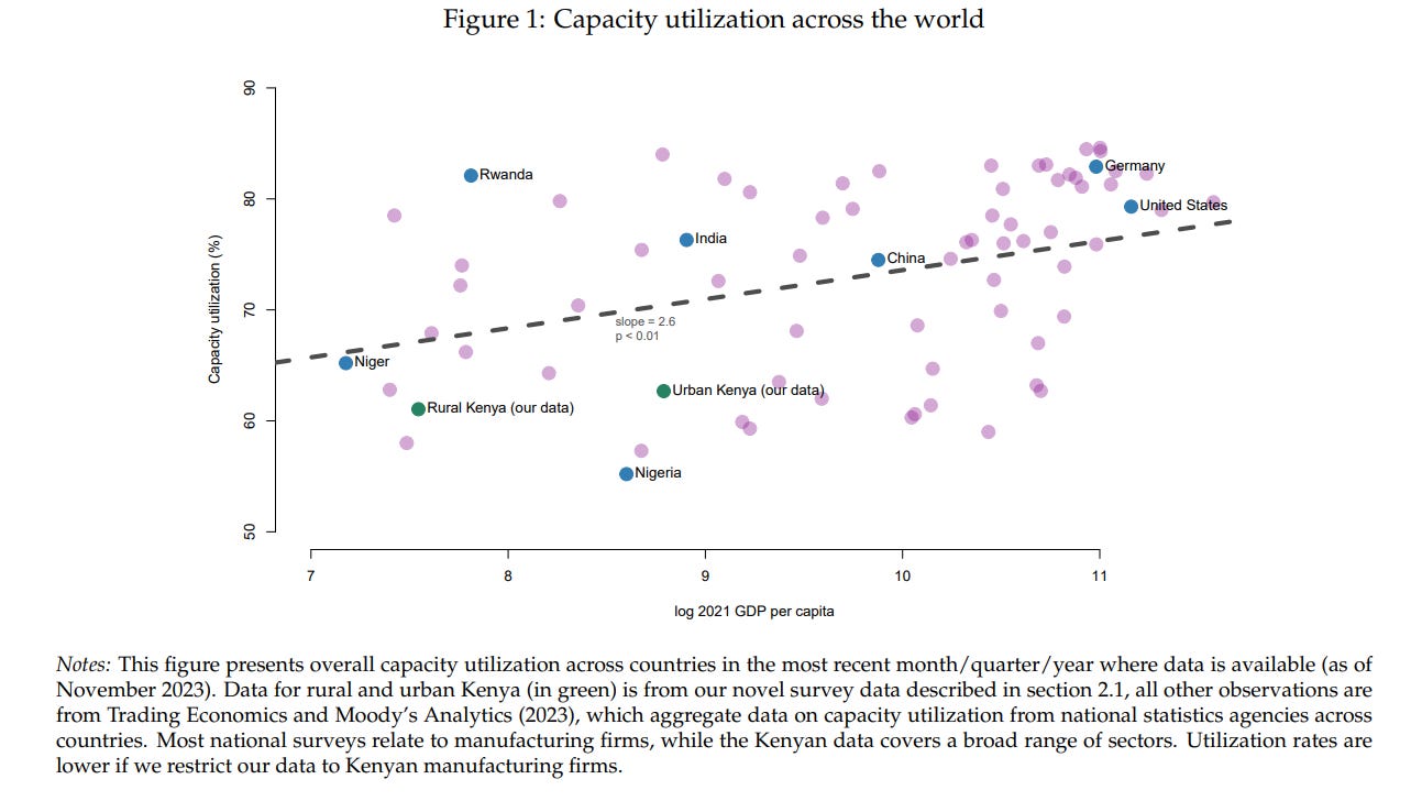
One of the more intriguing explanations comes from the team behind the GiveDirectly experiment – you can’t buy half a machine. You can only buy an integer. If demand isn’t there, you only run a machine part of the time, even though it could be run all of the time at little additional cost. A grain mill is a common example of this – if additional people lived there, or transportation became cheaper or demand were higher, you could support more usage. The poor countries of the world tend to (I believe this somewhat) use less of their productive capacity than the developed world.

And to be clear, this need not be just machines. A restaurant is most productive if it is serving people all of the time, rather than waiting around idly for customers. The GiveDirectly experiment people find that the most “slack” in production can be found in microenterprises with a single owner-employee, and in thinner markets in the country. Moving to the city, as discussed in Monday’s article, is a way of having customers around.

This is substantially different, by the way, from the famous Keynesian multiplier. You should not take from this that the central bank of Kenya should pursue a more expansionary monetary policy, nor would I say the government of Kenya should engage in fiscal stimulus. These are increasing returns to a real wealth shock, not a temporary fooling of the people. The money will never have to be clawed back in taxes or inflation.

What is an interesting puzzle is reconciling this with results on the effects of roads. If there is substantial slack in the utilization of inputs, then things which lower transportation costs should have fiscal multipliers. Asher and Novosad (2017), though, found that roads in rural India simply led to people leaving the countryside to go to the cities. Now, this need not be a bad thing. I’m inclined to think it’s quite good. Frankly it just goes to show the difficulty in aggregating together findings in different contexts.

I do not venture a guess as to whether cash transfers exceed the gains from public health initiatives like those favored by Givewell. Unfortunately, the question is fundamentally normative. It depends on how you weigh death against loss of consumption. However, if you do care about raising the consumption of the poorest of the poor, you can be assured that GiveDirectly is a good use of funds.